pt(q, df = your.df, lower.tail = FALSE) * 219 T-tests
Some simple hypothesis tests with the t statistic:
-
One sample t tests to contrasting a single sample parameter to a population parameter
- Independent samples t tests to contrast the means of two samples
- Paired t-tests to contrast two groups of values where each pair is measured from the same object.
19.1 One Sample T-test
One of the simplest hypothesis tests in statistics is to test whether a single parameter from a sample of measurements differs from a hypothesised population parameter. The test is asking what is the likelihood of obtaining that sample from a population with certain properties.
For this, we use a one sample t-test. The test statistic, t, has the general form of:
\[t = \frac{St-\theta}{S_{St}}\]
where St is the value of the statistic from your sample, \(\theta\) is the population value against which you are comparing your sample, and \(S_{St}\) is the standard error of your sample statistic.
Such tests can be used for a variety of parameters sampled from populations (e.g., means, slopes and intercepts in linear regression etc.). Here, lets look at a simple example where we test whether the mean of a set of replicated measures differs from a hypothesised value.

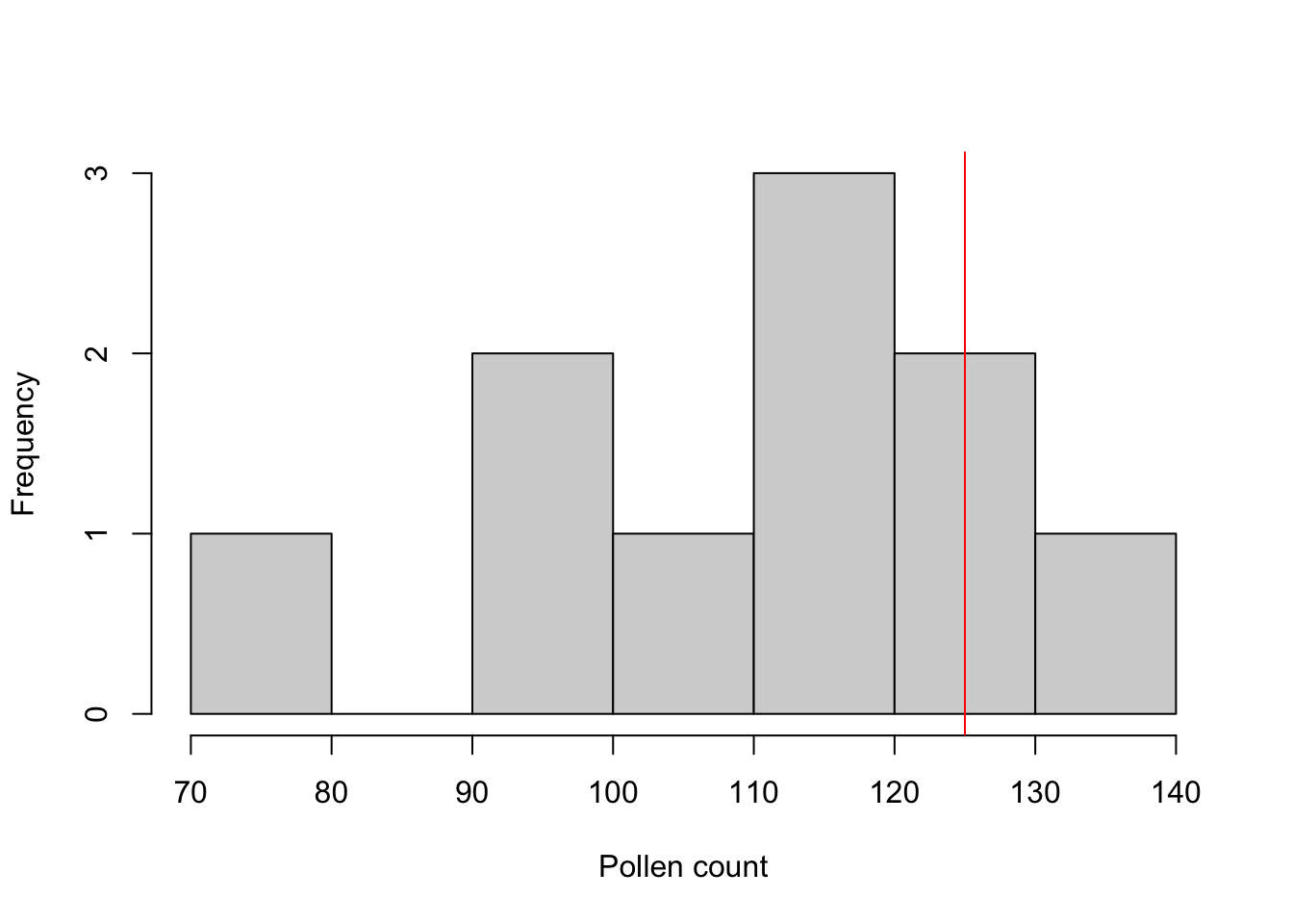
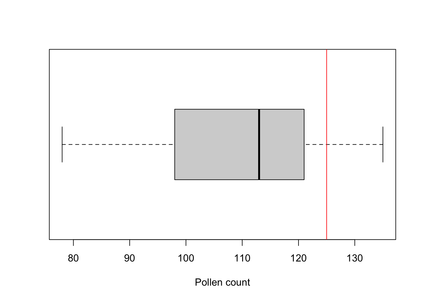
Imagine that a forensic scientist was trying to track the origin of some soil samples taken from footprints at a crime scene. She collected 10 samples and analysed the concentration of pollen from a species of pine tree found in a local forest. It was known that soil from that local forest had an average concentration of 125 grains per gram of soil. The one sample t-test will test the likelihood of the ten samples coming from that forest by contrasting the mean concentration in the ten new samples to the value expected if they came from that forest.
The test statistic, t is:
\[t = \frac{\bar{x}-\mu}{SE}\]
where \(\bar{x}\) is the sample mean, \(\mu\) is the population mean and SE is the standard error of the sample.
Note that the size of test statistic depends on two things: 1) how different the sample mean is to the population mean (the numerator) and 2) how much variation is present within the sample (the denominator). The null hypothesis is that the population mean from which the sample was taken is the known value, i.e., \(H_o: \mu=125\).
19.1.1 Running the analysis
The test statistic t is relatively straightforward to manually calculate. The test statistic can then checked against a t distribution in order to determine the probability of obtaining that value of the test statistic if the null hypothesis is true.
To calculate the probability associated with a given value of t in R, use
where q is your value of t, your.df is the degrees of freedom (n-1). The lower.tail = FALSE ensures that you are calculating the probability of getting a t value larger than yours (i.e., the upper tail, P[X > x]). Note that the critical value for \(t_{\alpha = 0.05}\) varies depending on the number of degrees of freedom - larger degrees of freedom = smaller critical value of t.
Much easier is to use the t.test function in R to give you the test statistic and its associated probability in one output. For a one sample t-test, we would use:
t.test(y, mu = your.mu)where y is a vector with your sample data and your.mu is the population parameter you are comparing the sample to.
For our crime scene example, we could assign our ten measurements to an object called pollen and run the t-test on that object.
19.1.2 Interpreting the results
    One Sample t-test

data:  pollen
t = -3.0691, df = 9, p-value = 0.01337
alternative hypothesis: true mean is not equal to 125
95 percent confidence interval:
  97.20685 120.79315
sample estimates:
mean of x
      109
The output of a one sample t-test is straight-forward to interpret. In the above output, the test statistic t = -3.0691 with 9 degrees of freedom, and a low p value (p = 0.013). We can therefore reject the null hypothesis and conclude that it was unlikely that the soil samples from the crime scene came from the nearby pine forest.
You also get the mean of your sample (109) and the 95% confidence interval for population mean estimated from that sample (this will not overlap your hypothesised mean when the test is significant).
19.1.3 Assumptions to check
t-tests are parametric tests, which implies we can specify a probability distribution for the population of the variable from which samples were taken. Parametric (and non-parametric) tests have a number of assumptions. If these assumptions are violated we can no longer be sure that the test statistic follows a t distribution, in which case p-values may be inaccurate.
Normality. The t distribution describes paramaters sampled from a normal population, so assumes that the data are normally distributed. Note however that t tests are reasonably robust to violations of normality (although watch out for the influence of outliers).
Independence. The observations should have been sampled randomly from a defined population so that sample mean is an unbiased estimate of the population mean. If individual replicates are linked in any way, then the assumption of independence will be violated.
19.1.4 Communicating the results
Written. As a minimum, the observed t statistic, the p value and the number of degrees of freedom should be reported. For example, you could write “The mean pollen count from the footprints (109 ) was significantly lower than expected if it was derived from the nearby forest with an average count of 125 (t = 3.07, df = 9, P = 0.01)”.
Visual. Box plots or frequency histograms can be used to visualise the variation in a single variable. In this example, you might use a line or arrow to indicate the single value (125) that you were comparing the sample to.
19.1.5 Further help
Type ?t.test to get the R help for this function.
Quinn and Keough (2002) Experimental design and data analysis for biologists. Cambridge University Press. Chapter 3: Hypothesis testing.
McKillup (2012) Statistics explained. An introductory guide for life scientists. Cambridge University Press. Chapter 9: Comparing the means of one and two samples of normally distributed data.
Author: Alistair Poore
Year: 2016
19.2 Two Sample T-test
An independent samples t-test aka a two sample t-test is one of the most commonly used statistical tests. It is used for comparing whether the means of two samples are statistically different from each other (e.g., control vs. treatment, site A vs site B etc). For example, consider the simple case of whether a sample of pH measurements from one river differs from a sample of pH measurements from a second river.

The null hypothesis is that the population means from which the two samples are taken are equal \[H_o: \mu_1=\mu_2\].
The test statistic, t, is:
\[t = \frac{\bar{x_{1}}-\bar{x_{2}}}{s_{\bar{y_{1}}-\bar{y_{2}}}}\]
where the denominator is the standard error of the difference between the two means.
\[\sqrt{\frac{(n_{1}-1)s_{1}^{2}+(n_{2}-1)s_{2}^{2}}{n_{1}+n_{2}-2}{(\frac{1}{n_{1}}}+\frac{1}{n_{2}})}\]
Note that the size of test statistic depends on two things: 1) how different the two means are (the numerator) and 2) how much variation is present within each sample (the denominator).
This equation is for the pooled variance t-test. For a separate variances t-test (also known as Welch’s t test), which does not assume equal variances, the denominator is:
\[\sqrt{\frac{s_1^2}{n_1}+\frac{s_2^2}{n_2}}\]
Note that a t test is a special case of a linear model with a single continuous response variable and a single categorical predictor variable that has two levels.
19.2.1 Running the analysis
An independent samples t-test can be run with the same t.test function as used for one sample or paired t-tests. For an independent samples t-test assuming equal variances, we would use:
t.test(x <- my_sample1, y = my_sample2, var.equal = TRUE)where my_sample1 and my_sample2 are vectors containing the measurements from each sample.
More commonly, we would use a data frame with the response and predictor variables as separate columns. You can then use a formula statement, y ~ x, to specify the response and predictor variables rather than the code above. Consider the simple example where you wanted to compare the pH of two rivers. Ten replicate pH measures were taken from each river.
Download the sample data set, River_pH.csv, and import into R.
River_pH <- read.csv(file = "data/River_pH.csv", header = TRUE)The t-test is run with the t.test function, with the arguments specifying the response variable (pH) to the left of the ~, the predictor variable (River_name) to the right of the ~, and the data frame to be used.
t.test(pH ~ River_name, data = River_pH, var.equal = TRUE)The argument var.equal = TRUE specifies that we are assuming equal variances. Note the default t-test argument for the alternative hypothesis is a two-tailed test. If you want to conduct a one-tailed test you must add an argument to the function specifying alternative = "greater" or alternative = "less".
19.2.2 Interpreting the results
    Two Sample t-test

data:  River_pH$pH by River_pH$River_name
t = 6.9788, df = 18, p-value = 1.618e-06
alternative hypothesis: true difference in means between group A and group B is not equal to 0
95 percent confidence interval:
 1.574706 2.931168
sample estimates:
mean in group A mean in group B
       8.661497        6.408560
The output of a t-test is straight-forward to interpret. In the above output, the test statistic t = 6.9788 with 18 degrees of freedom, and a very low p value (p < 0.001). We can therefore reject the null hypothesis that the two rivers have the same pH.
You also get the means from the two samples (needed to know which one is larger if the test is significant), and the 95% confidence interval for the difference between the two means (this will not overlap zero when the test is signficant).
19.2.3 Assumptions to check
t-tests are parametric tests, which implies we can specify a probability distribution for the population of the variable from which samples were taken. Parametric (and non-parametric) tests have a number of assumptions. If these assumptions are violated we can no longer be sure that the test statistic follows a t distribution, in which case p-values may be inaccurate.
Normality. The data are normally distributed. Note however that t tests are reasonably robust to violations of normality (although watch out for the influence of outliers).
Equal variance. The variances of each sample are assumed to be approximately equal. t tests are also reasonably robust to violations of equal variance if sample sizes are the same but can be problematic when sample sizes are very different.
In the event of unequal variances, it may be better to perform a Welch’s t test which does not assume equal variances. To conduct a Welch test in R, the var.equal argument in t.test function should be changed to var.equal=FALSE. This is in fact the default argument for t.test if not specified.
Independence. The observations should have been sampled randomly from the population so that the two sample means are unbiased estimates of the population means. If individual replicates are linked in any way, then the assumption of independence will be violated.
19.2.4 Communicating the results
Written. As a minimum, the observed t statistic, the P-value and the number of degrees of freedom should be reported. For example, you could write “the pH was significantly higher in River A than River B (independent samples t-test: t = 6.98, df = 18, P < 0.001)”.
Visual. Box plots or column graphs with error bars are effective ways of communicating the variation in a single continuous response variable versus a single categorical predictor variable.
boxplot(pH ~ River_name, data = River_pH, xlab = "River name", ylab = "pH")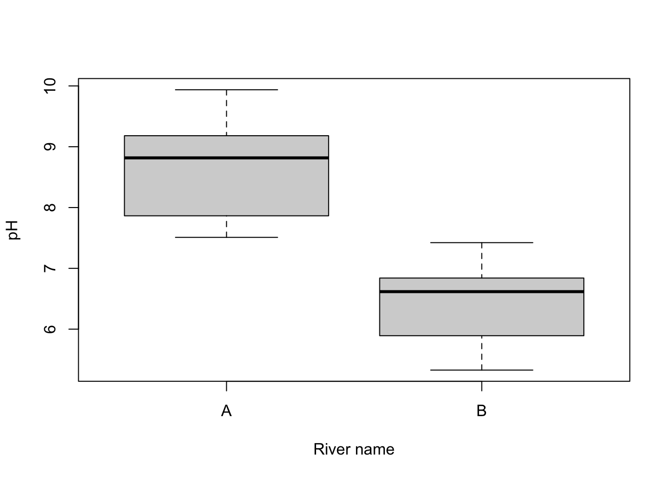
19.2.5 Further help
Type ?t.test to get the R help for this function.
Quinn and Keough (2002) Experimental design and data analysis for biologists. Cambridge University Press. Chapter 3: Hypothesis testing.
McKillup (2012) Statistics explained. An introductory guide for life scientists. Cambridge University Press. Chapter 9: Comparing the means of one and two samples of normally distributed data.
Author: Alistair Poore
Year: 2016
19.3 Paired T-test
Paired t-tests are used to compare the means of two groups of measurements when individual objects are measured twice, once for each type of measurement. Data could be paired in various ways: if the same measure is taken from a single object in two different treatments or at two different times, or if different types of measures are being contrasted from the same object.

For example, to contrast the photosynthetic performance of ten plants in two environments in a greenhouse (shady and sunny), we could measure performance in each individual plant twice, once in the shade and once in the sun. The measures are paired by belonging to the same individual plant.
For this experimental design, we would use a paired t-test to compare the measurements taken in the two environments. The 20 individual measurements are not independent of each other because we would expect the pair of measurements taken from the same individual to be more similar to each other than if randomly sampled from all available plants. We are thus unable to use an independent samples t test - that test would be appropriate if each plant was used only once, with some plants measured in the shady treatment and different set of plants measured in the sunny treatment.
Pairing data like this is usually done to reduce the likely variation among measurements with the aim of better detecting differences between groups. In this example, the difference between the two measures of photosynthetic performance on a given plant should reflect mostly the effect of sunlight, while in an independent samples design, the difference between a plant in the shade and another plant in the sun will reflect both differences in the effects of sunlight and differences between the individual plants.
For a paired t-test, the test statistic, t is:
\[t = \frac{\bar{d}}{SE_{d}}\]
Where the \(\bar{d}\) is the mean of the differences between values for each pair, and SEd is the standard error of that set of differences.
Note that this equation is identical to a one sample t-test, used to contrast any sample mean (\(\bar{x}\)) to a known population mean (\(\mu\)) or hypothesised value. What you are doing here is testing whether your sample of differences is likely to have come from a population of differences that have a mean of zero (another way of saying that your groups are the same).
\[t = \frac{\bar{x}-\mu}{SE}\]
19.3.1 Running the analysis
The test statistic t is relatively straightforward to calculate manually. The test statistic can then checked against a t distribution in order to determine the probability of obtaining that value of the test statistic if the null hypothesis is true. In R, to calculate the probability associated with a given value of t use:
pt(q, df = your.df, lower.tail = FALSE) * 2where q is your value of t, your.df is the degrees of freedom (the number of pairs-1). The lower.tail = FALSE ensures that you are calculating the probability of getting a t value larger than yours (i.e the upper tail, P[X > x]). Note that the critical value for t (\(\alpha = 0.05\)) varies depending on the number of degrees of freedom - larger degrees of freedom = smaller critical value of t.
The t.test function gives you the test statistic and its associated probability in one output. For an paired t-test, we would use:
t.test(x = my_sample1, y = my_sample2, paired = TRUE)where my_sample1 and my_sample2 are vectors containing the measurements from each sample. You would need to make sure the two vectors have the same number of values and that data from each pair were in the matching rows.
If your data frame has one row per measurement, with the response and treatment in separate columns, reshape it so that each pair occupies one row before running the paired test. Use the plant identifier to match measurements rather than relying on their row order.
Download a sample data set in this format, Greenhouse.csv, and import into R
Greenhouse <- read.csv(file = "data/Greenhouse.csv", header = TRUE)For the paired t-test, the two measurements from each plant need to be side by side, so we first reshape the data to have one row per plant and a column for each treatment (see reshaping data). The t.test function is then given the two columns and told that they are paired. (Older versions of R also allowed t.test(Performance ~ Treatment, data = Greenhouse, paired = TRUE); since R 4.4 this is an error.)
Greenhouse_wide <- tidyr::pivot_wider(Greenhouse, id_cols = Plant,
  names_from = Treatment, values_from = Performance
)
t.test(Greenhouse_wide$Sunny, Greenhouse_wide$Shady, paired = TRUE)
19.3.2 Interpreting the results
    Paired t-test

data:  Greenhouse_wide$Sunny and Greenhouse_wide$Shady
t = 18.812, df = 9, p-value = 1.557e-08
alternative hypothesis: true mean difference is not equal to 0
95 percent confidence interval:
 0.1658326 0.2111674
sample estimates:
mean difference
         0.1885
The important output of a paired t-test includes the test statistic t, in this case 18.8, the degrees of freedom (in this case 9) and the probability associated with that value of t. In this case, we have a very low p value (p < 0.001) and can reject the null hypothesis that the plants can photosynthesise with the same performance in the two light environments.
You also get the mean and 95% confidence intervals for the differences between measurements in each pair (this will not overlap zero when the test is significant).
19.3.3 Assumptions to check
t-tests are parametric tests, which implies we can specify a probability distribution for the population of the variable from which samples were taken. Parametric (and non-parametric) tests have a number of assumptions. If these assumptions are violated we can no longer be sure that the test statistic follows a t distribution, in which case p-values may be inaccurate.
Normality. For a paired t-test, it is assumed the the sample of differences is normally distributed. If these are highly skewed, transformations may be used to achieve a distribution closer to normal.
Independence. The paired design takes into account that the two measures from each pair are not independent. It is still important, however, that each pair of objects measured are independent from other pairs. If they are linked in any way (e.g., groups of plants sharing a water tray) then more complex analytical design that account for additional factors may be required.
19.3.4 Communicating the results
Written. As a minimum, the observed t statistic, the P-value and the number of degrees of freedom should be reported. For example, you could write “The photosynthetic performance of plants was significantly greater in sunny environments in contrast to shady environments (paired t-test: t = 18.81, df = 9, P < 0.001)”.
Visual. Box plots or column graphs with error bars are effective ways of communicating the variation in a single continuous response variable versus a single categorical predictor variable.
boxplot(Performance ~ Treatment, data = Greenhouse, xlab = "Light environment", ylab = "Photosynthetic performance (FvFm)")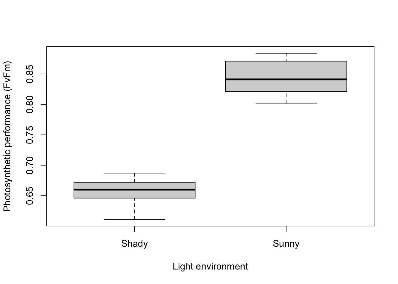
19.3.5 Further help
Type ?t.test to get the R help for this function.
Quinn and Keough (2002) Experimental design and data analysis for biologists. Cambridge University Press. Chapter 9: Hypothesis testing.
McKillup (2012) Statistics explained. An introductory guide for life scientists. Cambridge University Press. Chapter 9: Comparing the means of one and two samples of normally distributed data.
Author: Alistair Poore
Year: 2016