Data Types + Structure
One of the most common sources of frustration for beginners in R is dealing with different data structures and types. Here is an overview of the most important data structures, types and how to check and manipulate them.
The terms ‘structure’ and ‘type’ are often used interchangable. To avoid confusion, for this help page, data structure refers whether the data is a vector, matrix or data frame etc. and type refers to whether the data or variable is an integer, character or numeric etc.
One dimensional data (vectors)
The most basic data structure in R is a vector, a one-dimensional set of numbers or characters. This is the data structure that you will work with the most, albeit from within a data frame (see below). Vectors can be either atomic or list, atomic vectors differ to lists in that all elements within an atomic vector must be of the same type (see below). For the most part we work with atomic vector and the following help file refers to this type of data.
Common types of vectors
Common types of atomic vectors are logical, integer, numeric (i.e., double), character and factor. You can easily create each of these data types by using c(). In the integer example, the L forces R to consider those numbers as integers rather than numerical.
eg_logical <- c(T, T, T, F, F)
eg_integer <- c(1L, 6L, 1L, 5L, 4L)
eg_numeric <- c(0, 2.3, 2.45, 2.99, -1.1)
eg_character <- c("things", "in", "apostrophe", "are", "characters")
eg_factor <- factor(c("NSW", "NSW", "ACT", "WA", "WA"))
Factors (a special data type)
Notice how I couldn’t just use the c() to create a factor. Though factors look (and behave for the most part) like characters, they are actually a special type of integer with predefined categories, known as levels. The factor in this example has three levels: NSW, ACT and WA.
You can check how many levels any factor has using:
levels(eg_factor)## [1] "ACT" "NSW" "WA"This makes them behave differently to integers. Once created, factors can only contain a pre-defined set levels. For example, if you collecting data from sites across Australia you could have the fixed number of states as a factor, but it would be better to have a variable like site as a character if you were going to add data from more sites later on.
By default, R will always sort levels in alphabetical order. If you want your factors to be ordered (i.e., small, medium, high), use ordered to define the sequence you would like the levels to be presented. This is particularly useful for graphics to present the categories along an x axis in a more logical order.
sizes <- factor(c("small", "large", "large", "small", "medium"))
sizes
## [1] small  large  large  small  medium
## Levels: large medium small
sizes <- ordered(sizes, levels = c("small", "medium", "large"))
sizes
## [1] small  large  large  small  medium
## Levels: small < medium < large
See here for more info on ordered factors.
Checking data types
You can check the data type of any vector using the class or is functions.
class(eg_logical)
## [1] "logical"
is.integer(eg_integer)
## [1] TRUE
is.factor(eg_factor)
## [1] TRUE
Automatic coercion
As all elements within an atomic vector must be the same type, combining different types will coerce the data to the most flexible. Types from least to most flexible are: logical, integer, double, and character. For example, combining and integers and character will produce a character vector. This is something to be aware whilst manipulating your own data, especially when merging data frames.
eg_coerced <- c("tricks", 1, 2, 3, 4)
class(eg_coerced)
## [1] "character"
Coercing data
If you find your data is the wrong type, you can use the as functions to coerce data from one type to another. Be aware of what happens to your data after coercion. For example, coercing logical to numeric replaces F with 0s and Ts with 1s and any nonsensical coercion (like trying to make character “NSW” into a numeric) will result in NAs.
as.numeric(eg_logical)
## [1] 1 1 1 0 0
as.numeric(eg_character)
## Warning: NAs introduced by coercion
## [1] NA NA NA NA NA
Two dimensional data (matrices and data frames)
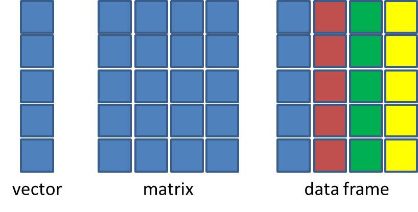
For the most part, we tend to work with two dimensional data containing both columns and rows. Like the one dimensional vectors, they come in two forms: matrices, where all vectors must be of all the same type of data, and data frames, which can be made up of vectors containing different data types.
Matrices
Matrices are easily constructed in R and can you check if its a matrix using the class function. For example, to make a matrix with 3 rows and 2 columns with 6 values:
eg_matrix <- matrix(c(1, 2, 3, 4, 5, 6), nrow = 3, ncol = 2)## [,1] [,2]
## [1,] 1 4
## [2,] 2 5
## [3,] 3 6Think of matrices as atomic vectors with dimensions; the number of rows and columns. Like atomic matrices, you can check the type of data with is and coerce using the as functions.
is.logical(eg_matrix)
## [1] FALSE
as.numeric(eg_logical)
## [1] 1 1 1 0 0
Data frames
The most common data structure we work with is the data frame. Data frames are just a collection of atomic vectors of equal length stuck together. They are different to matrices as they can contain vectors of different types.
To make a simple data frame that combines three of the vectors we made above, we could use:
eg_data_frame <- data.frame(eg_character, eg_factor, eg_numeric)## eg_character eg_factor eg_numeric
## 1 things NSW 0.00
## 2 in NSW 2.30
## 3 apostrophe ACT 2.45
## 4 are WA 2.99
## 5 characters WA -1.10More commonly, we import data entered into a spreadsheet straight into a data frame using read.csv (see help Importing data).
To check the data types within a data frame, use the str function. This gives an output listing for each column (i.e., variables) and the respective data type.
str(eg_data_frame)## 'data.frame': 5 obs. of 3 variables:
## $ eg_character: chr "things" "in" "apostrophe" "are" ...
## $ eg_factor : Factor w/ 3 levels "ACT","NSW","WA": 2 2 1 3 3
## $ eg_numeric : num 0 2.3 2.45 2.99 -1.1Note that data types can change. In this example, the character vector has been coerced to a factor in the process of making the data frame.
If you wish to check the data type of just one variable, or change that variable to another type, we use $ to access that variable from within the data frame. For example:
str(eg_data_frame$eg_character)
##  chr [1:5] "things" "in" "apostrophe" "are" "characters"
levels(eg_data_frame$eg_factor)
## [1] "ACT" "NSW" "WA"
is.numeric(eg_data_frame$numeric)
## [1] FALSE