One Sample T-test
One of the simplest hypothesis tests in statistics is to test whether a single parameter from a sample of measurements differs from a hypothesised population parameter. The test is asking what is the likelihood of obtaining that sample from a population with certain properties.
For this, we use a one sample t-test. The test statistic, t, has the general form of:
\[t = \frac{St-\theta}{S_{St}}\]
where St is the value of the statistic from your sample, \(\theta\) is the population value against which you are comparing your sample, and \(S_{St}\) is the standard error of your sample statistic.
Such tests can be used for a variety of parameters sampled from populations (e.g., means, slopes and intercepts in linear regression etc.). Here, lets look at a simple example where we test whether the mean of a set of replicated measures differs from a hypothesised value.

Imagine that a forensic scientist was trying to track the origin of some soil samples taken from footprints at a crime scene. She collected 10 samples and analysed the concentration of pollen from a species of pine tree found in a local forest. It was known that soil from that local forest had an average concentration of 125 grains per gram of soil. The one sample t-test will test the likelihood of the ten samples coming from that forest by contrasting the mean concentration in the ten new samples to the value expected if they came from that forest.
The test statistic, t is:
\[t = \frac{\bar{x}-\mu}{SE}\]
where \(\bar{x}\) is the sample mean, \(\mu\) is the population mean and SE is the standard error of the sample.
Note that the size of test statistic depends on two things: 1) how different the sample mean is to the population mean (the numerator) and 2) how much variation is present within the sample (the denominator). The null hypothesis is that the population mean from which the sample was taken is the known value, i.e., \(H_o: \mu=125\).
Running the analysis
The test statistic t is relatively straightforward to manually calculate. The test statistic can then checked against a t distribution in order to determine the probability of obtaining that value of the test statistic if the null hypothesis is true.
To calculate the probability associated with a given value of t in R, use
pt(q, df = your.df, lower.tail = FALSE) * 2where q is your value of t, your.df is the degrees of freedom (n-1). The lower.tail = FALSE ensures that you are calculating the probability of getting a t value larger than yours (i.e., the upper tail, P[X > x]). Note that the critical value for \(t_{\alpha = 0.05}\) varies depending on the number of degrees of freedom - larger degrees of freedom = smaller critical value of t.
Much easier is to use the t.test function in R to give you the test statistic and its associated probability in one output. For a one sample t-test, we would use:
t.test(y, mu = your.mu)where y is a vector with your sample data and your.mu is the population parameter you are comparing the sample to.
For our crime scene example, we could assign our ten measurements to an object called pollen and run the t-test on that object.
pollen <- c(94, 135, 78, 98, 137, 114, 114, 101, 112, 121)
t.test(pollen, mu = 125)
Interpreting the results
##
##  One Sample t-test
##
## data:  pollen
## t = -3.0691, df = 9, p-value = 0.01337
## alternative hypothesis: true mean is not equal to 125
## 95 percent confidence interval:
##   97.20685 120.79315
## sample estimates:
## mean of x
##       109
The output of a one sample t-test is straight-forward to interpret. In the above output, the test statistic t = -3.0691 with 9 degrees of freedom, and a low p value (p = 0.013). We can therefore reject the null hypothesis and conclude that it was unlikely that the soil samples from the crime scene came from the nearby pine forest.
You also get the mean of your sample (109) and the 95% confidence interval for population mean estimated from that sample (this will not overlap your hypothesised mean when the test is significant).
Assumptions to check
t-tests are parametric tests, which implies we can specify a probability distribution for the population of the variable from which samples were taken. Parametric (and non-parametric) tests have a number of assumptions. If these assumptions are violated we can no longer be sure that the test statistic follows a t distribution, in which case p-values may be inaccurate.
Normality. The t distribution describes paramaters sampled from a normal population, so assumes that the data are normally distributed. Note however that t tests are reasonably robust to violations of normality (although watch out for the influence of outliers).
Independence. The observations should have been sampled randomly from a defined population so that sample mean is an unbiased estimate of the population mean. If individual replicates are linked in any way, then the assumption of independence will be violated.
Communicating the results
Written. As a minimum, the observed t statistic, the p value and the number of degrees of freedom should be reported. For example, you could write “The mean pollen count from the footprints (109 ) was significantly lower than expected if it was derived from the nearby forest with an average count of 125 (t = 3.07, df = 9, P = 0.01)”.
Visual. Box plots or frequency histograms can be used to visualise the variation in a single variable. In this example, you might use a line or arrow to indicate the single value (125) that you were comparing the sample to.
hist(pollen, xlab = "Pollen count", main = NULL)
abline(v = 125, col = "red")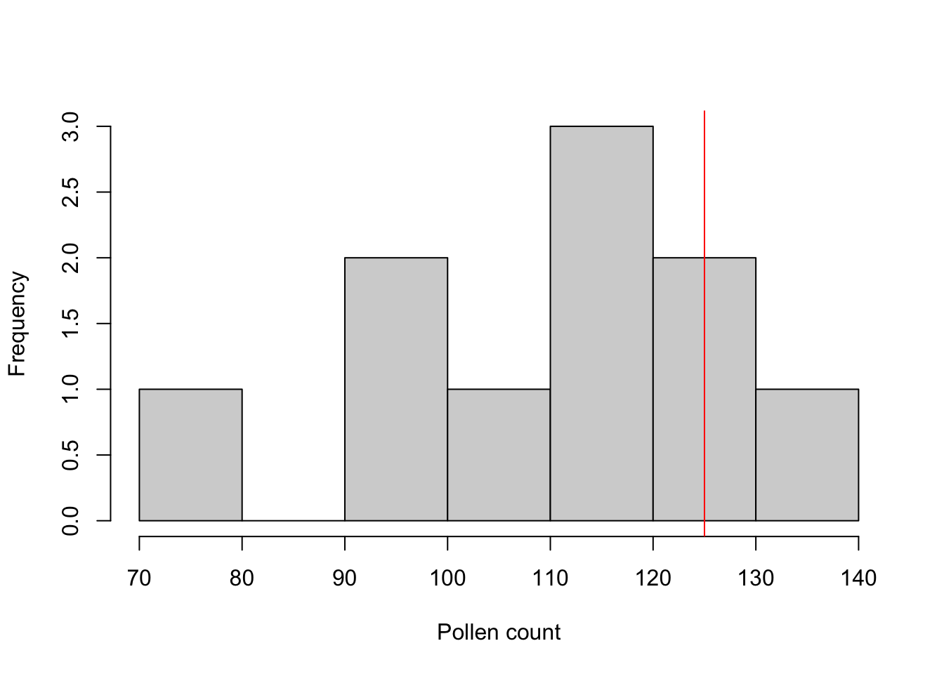
boxplot(pollen, xlab = "Pollen count", horizontal = TRUE)
abline(v = 125, col = "red")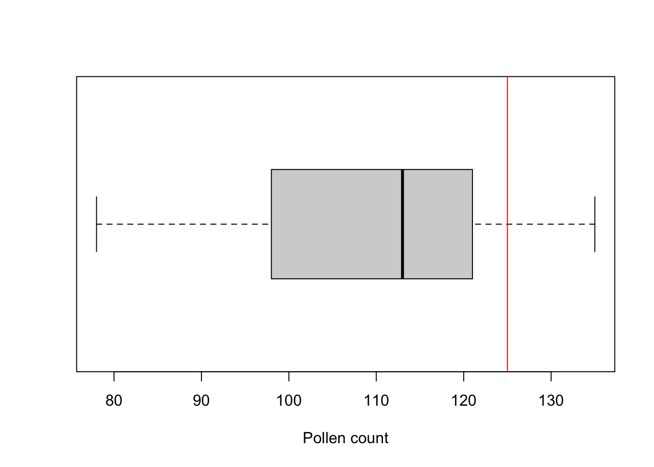
Further help
Type ?t.test to get the R help for this function.
Quinn and Keough (2002) Experimental design and data analysis for biologists. Cambridge University Press. Chapter 3: Hypothesis testing.
McKillup (2012) Statistics explained. An introductory guide for life scientists. Cambridge University Press. Chapter 9: Comparing the means of one and two samples of normally distributed data.
Author: Alistair Poore
Year: 2016
Last updated: Feb 2022