Count Data
Count data
This is a continuation of Generalised linear models 1 which introduced GLMs and gave instructions for binary data. Read that first to understand when GLMs are used. On this page, we will cover the use of GLM’s for count data and briefly introduce how they can be used for other data types you may have.
Running the analysis
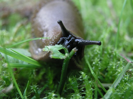
For this worked example, we have counts of different animal groups at control sites and sites where bush regeneration has been carried out (treatment). We want to know if the the bush regeneration activities have affected the count of slugs.
Download the sample data set, Revegetation.csv, and import into R to see how the data are arranged:
Reveg <- read.csv("Revegetation.csv", header = T)If you view the frequency histogram of the slug counts, you will see that it is very skewed, with many small values and few large counts (the variable name, Soleolifera, is the order name of terrestrial slugs).
hist(Reveg$Soleolifera)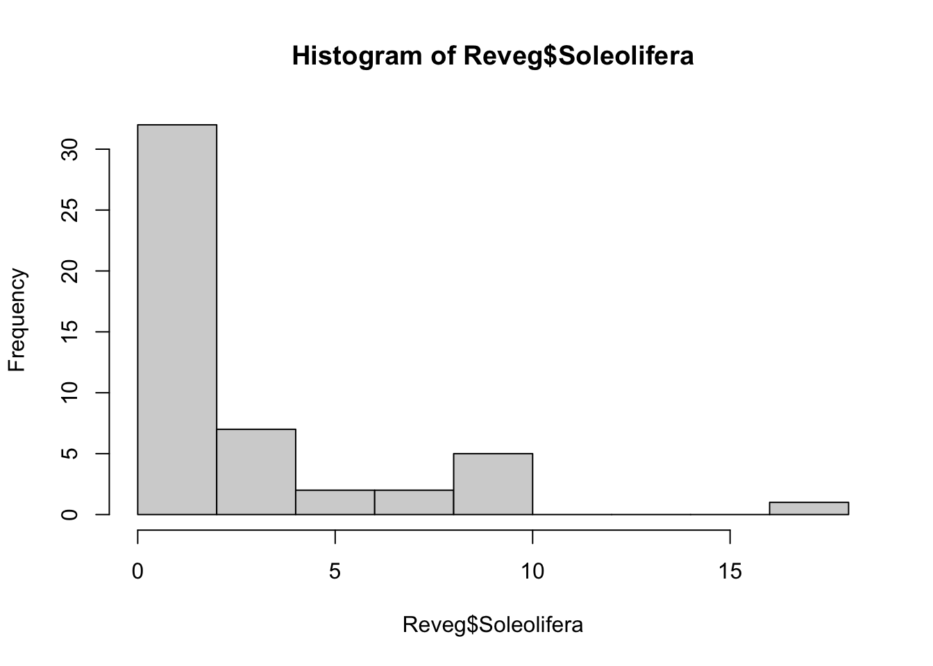
The default distribution for count data is the Poisson. The Poisson distribution assumes the variance equals the mean. This is quite a restrictive assumption which ecological count data often violate. We may need to use the more flexible negative-binomial distribution instead.
We can use a GLM to test whether the counts of slugs (from the order Soleolifera) differ between control and regenerated sites. To fit the GLM, we will use the manyglm function instead of glm so we have access to more useful residual plots.
To fit the GLM, load the mvabund package then fit the following model:
library(mvabund)
ft.sol.pois <- manyglm(Soleolifera ~ Treatment, family = "poisson", data = Reveg)
where Soleolifera is the response variable, and Treatment is the predictor variable (with two levels, control and revegetated).
Assumptions to check
Before we look at the results, we need to look at the residual plot to check the assumptions.
plot(ft.sol.pois)## Warning in default.plot.manyglm(x, res.type = res.type, which = which, caption =
## caption, : Only the first 1 colors will be used for plotting.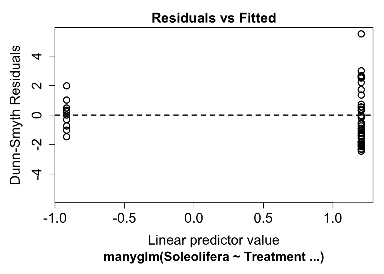
It’s hard to say whether there is any non-linearity in this plot, this is because the predictor is binary (treatment vs revegetated). Looking at the variance assumption, it does appear as though there is a fan shape. The residuals are more spread out on the right than the left - we call this overdispersion.
This tells us the variance assumption of the Poisson may be too restrictive and we should try a different distribution. We can instead fit a negative-binomial distribution in manyglm by changing the family argument to family="negative binomial".
ft.sol.nb <- manyglm(Soleolifera ~ Treatment, family = "negative binomial", data = Reveg)Look again at the residual plot:
plot(ft.sol.nb)## Warning in default.plot.manyglm(x, res.type = res.type, which = which, caption =
## caption, : Only the first 1 colors will be used for plotting.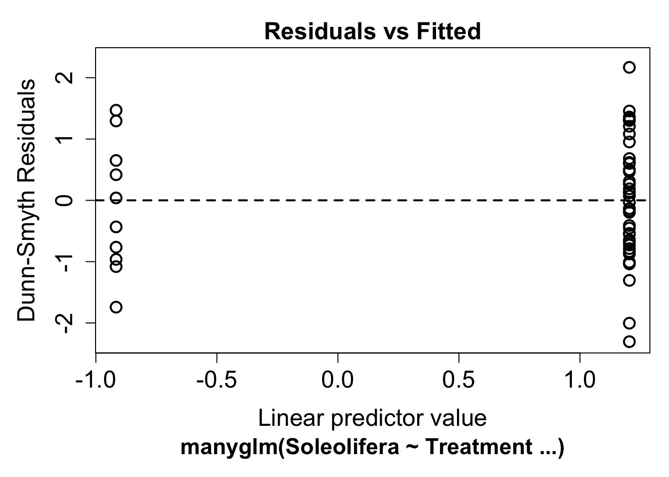
This seems to have improved the residual plot. There is no longer a strong fan shape, so we can go ahead and look at the results.
Interpreting the results
If all the assumption checks are okay, we can have a look at the results the model gave us with the same two functions for inference as used for linear models: summary and anova.
anova(ft.sol.nb)## Time elapsed: 0 hr 0 min 0 sec## Analysis of Deviance Table
##
## Model: Soleolifera ~ Treatment
##
## Multivariate test:
## Res.Df Df.diff Dev Pr(>Dev)
## (Intercept) 48
## Treatment 47 1 10.52 0.002 **
## ---
## Signif. codes: 0 '***' 0.001 '**' 0.01 '*' 0.05 '.' 0.1 ' ' 1
## Arguments: P-value calculated using 999 iterations via PIT-trap resampling.summary(ft.sol.nb)##
## Test statistics:
## wald value Pr(>wald)
## (Intercept) 1.502 0.023 *
## TreatmentRevegetated 3.307 0.001 ***
## ---
## Signif. codes: 0 '***' 0.001 '**' 0.01 '*' 0.05 '.' 0.1 ' ' 1
##
## Test statistic: 3.307, p-value: 0.001
## Arguments: P-value calculated using 999 resampling iterations via pit.trap resampling.Both tests indicate strong evidence of a treatment effect (p<0.01). To extract the model equation we can look at the coefficients from the fit.
ft.sol.nb$coefficients## Soleolifera
## (Intercept) -0.9162907
## TreatmentRevegetated 2.1202635The default link function for Poisson and negative binomial models is \(log()\). If we write the mean count as \(\lambda\)
\[ \log(\lambda) = -0.92 + 2.12 \times \text{Treatment}\]
Communicating the results
Written. Results of GLM’s are communicated in the same way as results for linear models. For one predictor it suffices to write one line, e.g. “There is strong evidence of positive effect of bush regeneration on the abundance of slugs from the order Soleolifera (p < 0.001)”. For multiple predictors it’s best to display the results in a table. You should also indicate which distribution was used (e.g. negative-binomial) and if resampling was used for inference. ” We used a negative-binomial generalised linear model due to overdispersion evident in the data. Inference was carried out using bootstrap resampling with 1000 resamples (default when using manyglm).”
Visual. In this example, a boxplot would be an effective way to visualse the differences in slug counts between control and revegetated sites.
boxplot(Soleolifera ~ Treatment, ylab = "Count", xlab = "Treatment", data = Reveg)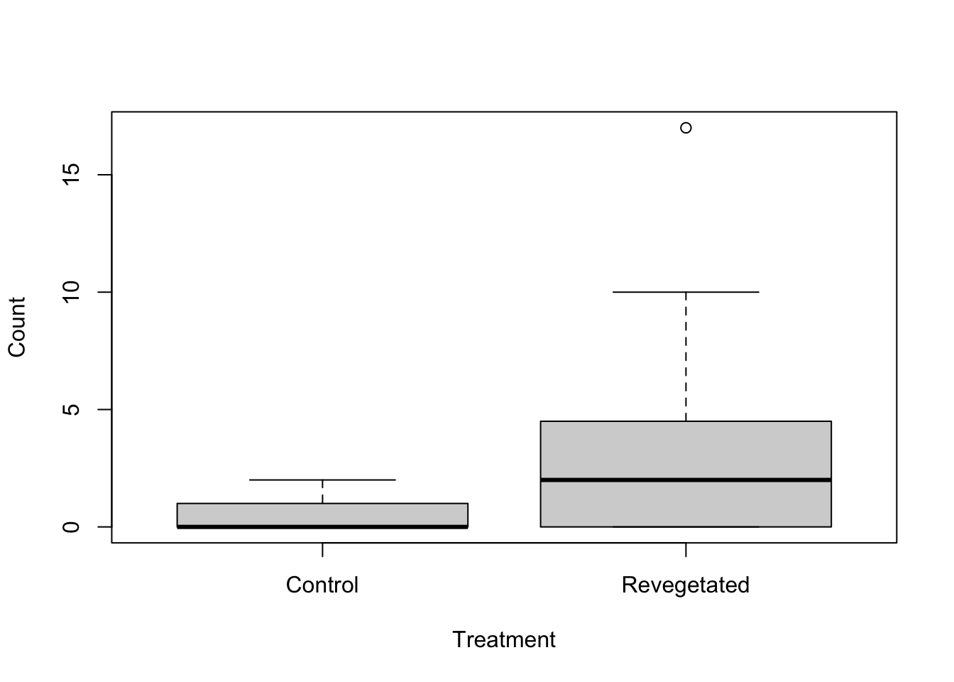
Other types of data
If you have continuous positive data with zeros, like biomass data, the tweedie distribution might be able to model this, although it does have some quite restrictive assumptions. You can use family="tweedie" with the manyglm function. Be sure to look at residual plots for violations of assumptions.
For strictly positive continuous data a gamma distribution can be used. This is available in the glm function using family=gamma.
Further help
You can type ?glm and ?manyglm into R for help with these functions.
Faraway, JJ. 2005. Extending the linear model with R: generalized linear, mixed effects and nonparametric regression models. CRC press.
Zuur, A, EN Ieno and GM Smith. 20074. Analysing ecological data. Springer Science & Business Media, 2007.
More advice on interpreting coefficients in glms
Author: Gordana Popovic
Year: 2016
Last updated: Feb 2022