Introduction
Linear mixed models with one random effect
You will need to use mixed effect models if you have a random factor in your experimental design. A random factor
- is categorical
- has a large number of levels
- only a random subsample of levels is included in your design
- you want to make inference in general, and not only for the levels you observed.
This is a tough concept to get your head around, and is best explained with an example. The data we will analyse here are counts of invertebrates at 3-4 sites in each of 7 (randomly chosen) estuaries. Here the estuaries are the random effect, as there are a large number of possible estuaries, and we only sample from a random few of them, but we would like to make inference about estuaries in general.

We will introduce mixed models in three parts
Mixed models 1 (this page) is an introduction to mixed models for a continuous response with one random effect. You will learn how to check assumptions and do inference, including the parametric bootstrap.
Mixed models 2 extends this to multiple random effects with a continuous response. We look into how to model nested and crossed random effects.
Mixed models 3 teaches you how to model discrete data, including counts and binary data, with random effects.
All three pages will use the same data for illustration.
Properties of mixed models
Assumptions. Mixed models make some important assumptions (we’ll check these later for our examples)
- The observed \(y\) are independent, conditional on some predictors \(x\)
- The response \(y\) are normally distributed conditional on some predictors \(x\)
- The response \(y\) has constant variance, conditional on some predictors \(x\)
- There is a straight line relationship between \(y\) and the predictors \(x\) and random effects \(z\)
- Random effects \(z\) are independent of \(y\).
- Random effects \(z\) are normally distributed
Running the analysis
We will use the package lme4 for all our mixed effect modelling. It will allow us to model both continuous and discrete data with one or more random effects. First, install and load this package:
library(lme4)We will analyse a data set that aimed to test the effect of water pollution on the abundance of some subtidal marine invertebrates by comparing samples from modified and pristine estuaries. As the total counts are large, we will assume the data is continuous. Later on in Mixed models 3, we’ll model counts as discrete using Generalised linear mixed models (GLMMs).
Download the sample data set, Estuaries.csv, and load into R.
Estuaries <- read.csv("Estuaries.csv", header = T)Fitting a model with a fixed and random effect
In this data set, we have a fixed effect (Modification; modified vs pristine) and a random effect (Estuary). We can use the lmer function to fit a model for any dependent variables with a continuous distribution. To fit a model for total abundance, we would use:
ft.estu <- lmer(Total ~ Modification + (1 | Estuary), data = Estuaries, REML = T)where Total is the dependent variable (left of the ~), Modification is the fixed effect, and Estuary is the random effect.
Note the syntax for one random effect is (1|Estuary) - this is fitting a different intercept (hence 1) for each Estuary.
This model can be fit by maximum likelihood (REML=F) or restricted maximum likelihood (>REML=T). For fitting models it’s best to use REML, as it is less biased (unbiased for balanced samples), particularly in small samples. However to use the anova function below we need to refit with maximum likelihood.
Assumptions to check
Before we look at the results of our analysis, it’s important to check that our data met the assumptions of the model we used. Let’s look at all the assumptions in order.
Assumption 1: The observed \(y\) are independent, conditional on some fixed effects \(x\) and random effects \(z\)
We can’t check this assumption, but you can ensure it’s true by taking a random sample within each level of the random effect in your experimental design.
Assumption 2: The response \(y\) are normally distributed conditional on some predictors \(x\) and random effects \(z\)
This assumption is only critical when we have a small sample size or very skewed data. We can check it with a normal quantile plot of residuals.
qqnorm(residuals(ft.estu))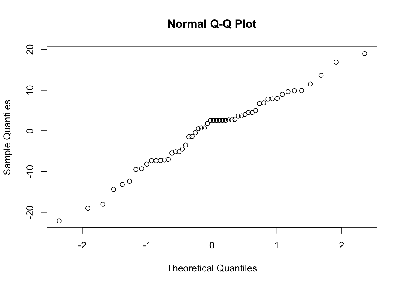
We are looking for a straight line relationship. Here, the assumption of normality seems reasonable.
Assumption 3: The response \(y\) has constant variance, conditional on some fixed effects \(x\) and random effects \(z\)
Like a linear model, a mixed model assumes constant variance. We can check this by looking for a fan shape in the residual plot (residuals vs fitted values).
scatter.smooth(residuals(ft.estu) ~ fitted(ft.estu))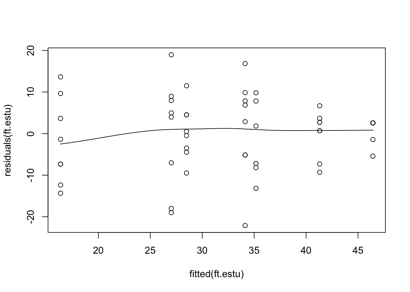
This residual plot seems reasonable, there are differences in variability between estuaries, but variability does not increase with the mean. Note, that the function scatter.smooth is just a scatter plot with a fitted, smoothed curve.
Assumption 4: There is a straight line relationship between \(y\) and the predictors \(x\) and random effects \(z\)
To check this assumption, we check the residual plot again for non-linearity, or a U-shape. In our case there is no evidence of non-linearity. If the residuals seem to go down then up, or up then down, we may need to add a polynomial function of the predictors using the poly function.
Assumption 5: Random effects \(z\) are independent of \(y\).
We can’t check this assumption, but you can ensure it’s true by taking a random sample of estuaries.
Assumption 6: Random effects \(z\) are normally distributed.
This assumption is not crucial (and difficult) to check.
Interpreting the results
Hypothesis test for the fixed effect
The package lme4 won’t give you p-values for fixed effects as part of the output in summary. This is because the p-values from Wald tests (using summary) and likelihood ratio tests (using anova) are only approximate in mixed models.
Nevertheless, we will use the anova function to test for an effect of modification on the total abundance of invertebrates, taking into account the random effect of estuary.
First, we fit the full model by maximum likelihood, and a second model that lacks the fixed effect of Modification
ft.estu <- lmer(Total ~ Modification + (1 | Estuary), data = Estuaries, REML = F)
ft.estu.0 <- lmer(Total ~ (1 | Estuary), data = Estuaries, REML = F)
Then, we compare these two models with a likelihood ratio test, using the anova function.
anova(ft.estu.0, ft.estu)## Data: Estuaries
## Models:
## ft.estu.0: Total ~ (1 | Estuary)
## ft.estu: Total ~ Modification + (1 | Estuary)
## npar AIC BIC logLik deviance Chisq Df Pr(>Chisq)
## ft.estu.0 3 415.02 420.99 -204.51 409.02
## ft.estu 4 411.92 419.87 -201.96 403.92 5.1055 1 0.02385 *
## ---
## Signif. codes: 0 '***' 0.001 '**' 0.01 '*' 0.05 '.' 0.1 ' ' 1We find that there is evidence of an effect of Modification (p = 0.02385).
We can also calculate confidence intervals for each model parameter using the confint function.
confint(ft.estu)## Computing profile confidence intervals ...## 2.5 % 97.5 %
## .sig01 2.718166 12.538348
## .sigma 7.676352 11.522837
## (Intercept) 31.918235 49.981321
## ModificationPristine -26.360731 -2.538241This also provides evidence for an effect of Modification as this parameter (i.e., the difference between the modified and pristine estuaries) has 95% confidence intervals that do not overlap zero.
Hypothesis test for random effects
You can use the anova function to test for random effects, but the p-values are very approximate and we do not recommend this procedure. Instead we will use a parametric bootstrap. This is a simulation based method which involves a fair chunk of code, but there’s not much about the code you have to change for different models, it’s mostly just a matter of copy-paste.
Parametric bootstrap
nBoot <- 1000
lrStat <- rep(NA, nBoot)
ft.null <- lm(Total ~ Modification, data = Estuaries) # null model
ft.alt <- lmer(Total ~ Modification + (1 | Estuary), data = Estuaries, REML = F) # alternate model
lrObs <- 2 * logLik(ft.alt) - 2 * logLik(ft.null) # observed test stat
for (iBoot in 1:nBoot)
{
  Estuaries$TotalSim <- unlist(simulate(ft.null)) # resampled data
  bNull <- lm(TotalSim ~ Modification, data = Estuaries) # null model
  bAlt <- lmer(TotalSim ~ Modification + (1 | Estuary), data = Estuaries, REML = F) # alternate model
  lrStat[iBoot] <- 2 * logLik(bAlt) - 2 * logLik(bNull) # resampled test stat
}
mean(lrStat > lrObs) # P-value for test of Estuary effect
## [1] 0.001There is strong evidence for including estuary in your model (p = 0.001). You could use similar code to test for the effect of Modification with a parametric bootstrap.
###FAQ for mixed models
1. Do I need balanced samples to fit a mixed model?
No, unbalanced designs are fine. Balanced designs will generally give you better power though, so they are good to aim for.
2. Should I sample many levels of the random effect, or lots of observations within each level?
This depends on what you are interested in. In our example, we are interested in the effect of modification. In the study design, estuaries fall directly below modification, so we need a lot of estuaries within each level of Modification to make good inference about the effects of modification. This is true in general, you need lots of samples in the level below the level you are primarily interested in.
3. Does my random factor have to be a random effect?
Not necessarily. If you have a random factor (i.e., you have a random sample of categories from a categorical variable) and you want to make inferences about that variable in general, not just at the categories you observed, then include it as a random effect. If you are happy making inference about just the levels you observed, then you can include it as a fixed effect. In our example we wanted to make inference about modification in general, i.e. in every modified and unmodified estuary, so we included estuary as a random effect. If we had treated Estuary as a fixed factor, we would have been restricted to making conclusions about only the estuaries we sample.
4. What if the levels of my factor aren’t really random?
This might be a problem as assumption 4 may not hold. You should always sample the random effect randomly to avoid bias and incorrect conclusions.
Communicating the results
Written. Results of linear mixed models are communicated in a similar way to results for linear models. In your results section you should mention that you are using mixed models with R package lme4, and list your random and fixed effects. You should also mention how you carried out inference, i.e. likelihood ratio tests (using the anova function) or parametric bootstrap. In the results section for one predictor, it suffices to write one line, e.g. “There is strong evidence (p<0.001) of negative effect of modification on total abundance. For multiple predictors it’s best to display the results in a table.
Visual. The best way to visually communicate results will depend on your question, for a simple mixed model with one random effect, a plot of the raw data with the model means superimposed is one possibility. There is a little bit of code that is required for such a plot, and it will be a little different for your data and model.
ModEst <- unique(Estuaries[c("Estuary", "Modification")]) # find which Estuaries are modified

# Prepare a vector of colors with specific color by modification levels
myColors <- ifelse(unique(ModEst$Modification) == "Modified", rgb(0.1, 0.1, 0.7, 0.5),
  ifelse(unique(ModEst$Modification) == "Pristine", rgb(0.8, 0.1, 0.3, 0.6),
    "grey90"
  )
)

boxplot(Total ~ Estuary, data = Estuaries, col = myColors, xlab = "Estuary", ylab = "Total invertebrates")
legend("bottomleft",
  inset = .02,
  c(" Modified ", " Pristine "), fill = unique(myColors), horiz = TRUE, cex = 0.8
)

# 0 if Modified, 1 if Pristine
is.mod <- ifelse(unique(ModEst$Modification) == "Modified", 0,
  ifelse(unique(ModEst$Modification) == "Pristine", 1, NA)
)

Est.means <- coef(ft.estu)$Estuary[, 1] + coef(ft.estu)$Estuary[, 2] * is.mod # Model means
## Warning in coef(ft.estu)$Estuary[, 2] * is.mod: longer object length is not a
## multiple of shorter object lengthstripchart(Est.means ~ sort(unique(Estuary)), data = Estuaries, pch = 18, col = "red", vertical = TRUE, add = TRUE)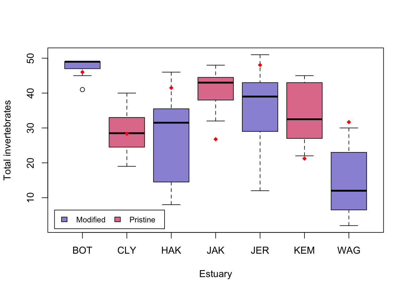
Further help
You can type ?lmer into R for help with these functions.
Draft book chapter from the authors of lme4.
Faraway, JJ. Extending the linear model with R: generalized linear, mixed effects and nonparametric regression models. CRC press, 2005.
Zuur, A, EN Ieno and GM Smith. Analysing ecological data. Springer Science & Business Media, 2007.
Author: Gordana Popovic
Year: 2016
Last updated: Feb 2022