Single Factor ANOVA
Analysis of variance (ANOVA) is one of the most frequently used techniques in the biological and environmental sciences. ANOVA is used to contrast a continuous dependent variable y across levels of one or more categorical independent variables x. The independent variables are termed the factor or treatment, and the various categories within that treatment are termed the levels. In this module, we will start with the simplest design - those with a single factor.
Where an independent samples t-test would be used for comparison of group means across two levels, ANOVA is used for the comparison of >2 group means, or when there are more than two or more predictor variables (see ANOVA: factorial). The logic of this test is essentially the same as the t-test - it compares variation between groups to variation within groups to determine whether the observed differences are due to chance or not.

For example, to contrast the the hatching times of turtle eggs incubated at four different temperatures (15°C, 20°C, 25°C and 30°C), hatching time is the continuous response variable and temperature is the categorical predictor variable with with four levels. The null hypothesis would be that mean hatching time is equal for all temperatures (Ho: \(\mu_{15} = \mu_{20} = \mu_{25} = \mu_{30}\)).
Note that an ANOVA is a linear model, just like linear regression except that the predictor variables are categorical rather than continuous.
\[y_{ij} = \mu + \alpha_i + \varepsilon_{ij}\]
where \(\mu\) is the overall mean and \(\alpha_i\) is the effect of the ith group.
It is the same as a multiple linear regression with a predictor variable for each level of the categorical variable (each coded as a dummy variable). For the question of whether hatching time of turtles differs between four incubation tempeatures, we must fit four parameters to describe the mean response of each temperature (rather than just a single intercept and single slope in a simple linear regression). For this example, our linear model equation will have this form:
\[HatchingTime = \mu + \beta_1.Temp_{15} + \beta_2.Temp_{20} + \beta_3.Temp_{25} + \beta_4.Temp_{30} + \varepsilon\]
ANOVA partitions the total variance into a component that can be explained by the predictor variable (among levels of the treatment), and a component that cannot be explained (within levels, the residual variance). The test statistic, F, is the ratio of these two sources of variation.
\[F = \frac{MS_{among}}{MS_{within}}\]
where MS are the mean squares, a measure of variation. The probability of obtaining the observed value of F is calculated from the known probability distribution of F, with two degrees of freedom (one for the numerator = the number of levels -1) and one for the denominator (number of replicates per level - 1 x number of levels).
Running the analysis
The data should be formatted such that the individual replicates are rows and the variables are separate columns. Include a column for the dependent variable, y, and a corresponding column for the categorical variable, x. Download the sample data set for the turtle hatching example, Turtles.csv, import into R and check that temperature variable is a factor with the str function.
Turtles <- read.csv(file = "Turtles.csv", header = TRUE)
str(Turtles)
In this case, because we have numbers for the four levels of the Temperature treatment, we need to change that variable to become a factor rather than an integer.
Turtles$Temperature <- factor(Turtles$Temperature)Now, we can run the analysis of variance contrasting hatching time (days) across temperatures using the function aov. The arguments of the function are simply a formula statement, y~x, with the response variable to the left of the ~, the predictor variable to the right, and some code to specify which data frame holds those variables.
Turtles.aov <- aov(Days ~ Temperature, data = Turtles)The output from this analysis can be seen by using the summary function on the object created.
summary(Turtles.aov)Exactly the same analysis can be reproduced using the linear model function lm.
Turtles.lm <- lm(Days ~ Temperature, data = Turtles)
summary(Turtles.lm)
Interpreting the results
##             Df Sum Sq Mean Sq F value   Pr(>F)
## Temperature  3   8025  2675.2   15.98 9.08e-07 ***
## Residuals   36   6027   167.4
## ---
## Signif. codes:  0 '***' 0.001 '**' 0.01 '*' 0.05 '.' 0.1 ' ' 1
The summary output of an ANOVA object is a table with the degrees of freedom (Df), sums of squares (Sum Sq), mean squares (Mean Sq) for the predictor variable (i.e., variation among levels of your treatment) and for the Residuals (i.e., varation within the levels). The test statistic, F value and its associated p-value (Pr(>F)) are also presented.
First check the degrees of freedom. The factor Df = the number of levels of your factor - 1. The residual Df = a(n-1), where a = the number of levels of your factor and n = sample size (replicates per level).
The sums of squares and mean squares are measures of variation. The F statistic is the ratio of MSamong and MSwithin and the p-value is the probability of the observed F value from the F distribution (with the given degrees of freedom).
The main thing to look at in the ANOVA table is whether your predictor variable had a significant effect on your response variable. In this example, the probability that all four incubation temperatures are equal is <0.001. This is very unlikely and much less than 0.05. We would conclude that there is a difference in hatching times between the temperatures. We are also interested in the R^2 value which tells us how much variation was explained by the model.
If you use the lm function, you get a bit more information from the summary of the linear model output.
##
## Call:
## lm(formula = Days ~ Temperature, data = Turtles)
##
## Residuals:
##     Min      1Q  Median      3Q     Max
## -28.200  -9.225   1.650   9.025  19.400
##
## Coefficients:
##               Estimate Std. Error t value Pr(>|t|)
## (Intercept)     58.400      4.092  14.273  < 2e-16 ***
## Temperature20  -13.800      5.787  -2.385   0.0225 *
## Temperature25   -9.200      5.787  -1.590   0.1206
## Temperature30  -38.300      5.787  -6.619 1.04e-07 ***
## ---
## Signif. codes:  0 '***' 0.001 '**' 0.01 '*' 0.05 '.' 0.1 ' ' 1
##
## Residual standard error: 12.94 on 36 degrees of freedom
## Multiple R-squared:  0.5711, Adjusted R-squared:  0.5354
## F-statistic: 15.98 on 3 and 36 DF,  p-value: 9.082e-07
The output for the standard ANOVA table is down the bottom and above it you get the actual parameter estimates from the linear model (the \(\beta_1\), \(\beta_2\) etc from above). In this example, turtles at 15°C hatched after 58.4 days, on average (the intercept in the model). The other parameter estimates are differences between each level of temperature and the intercept. For example, at 20°C they were 13.8 days faster (i.e., the mean for 20°C = 58.4-13.8 = 44.6 days).
If you detect any significant differences in the ANOVA, we are then interested in knowing exactly which groups differ from one another, and which do not. Remember that a significant p value in the test you just ran would reject the null hypothesis the means of the dependent variable were the same across all groups, but not identify which were different from each other. To see a comparison between each mean and each other mean, we can use a Tukey’s post-hoc test.
TukeyHSD(Turtles.aov)## Tukey multiple comparisons of means
## 95% family-wise confidence level
##
## Fit: aov(formula = Days ~ Temperature, data = Turtles)
##
## $Temperature
## diff lwr upr p adj
## 20-15 -13.8 -29.38469 1.784689 0.0982694
## 25-15 -9.2 -24.78469 6.384689 0.3969971
## 30-15 -38.3 -53.88469 -22.715311 0.0000006
## 25-20 4.6 -10.98469 20.184689 0.8562615
## 30-20 -24.5 -40.08469 -8.915311 0.0008384
## 30-25 -29.1 -44.68469 -13.515311 0.0000785Assumptions to check
The important assumptions of ANOVA are independence, homegeneity of variance and normality. We advocate a qualitative evalutation of the normality and homogeneity of variance assumptions, by examining the patterns of variation in the residuals, rather than a formal test such has Cochran’s test. Linear models in general are quite ‘robust’ for violating these assumptions (heterogeneity and normality), within reason.
Normality. The assumption of normality can be checked by a frequency histogram of the residuals or by using a quantile plot where the residuals are plotted against the values expected from a normal distribution. The histogram of residuals should follow a normal distribution. If the points in the quantile plot lie mostly on the line, the residuals are normally distributed. Both of these plots can be obtained from the model object created by the aov function.
par(mfrow = c(1, 2)) # This code put two plots in the same window
hist(Turtles.aov$residuals)
plot(Turtles.aov, which = 2)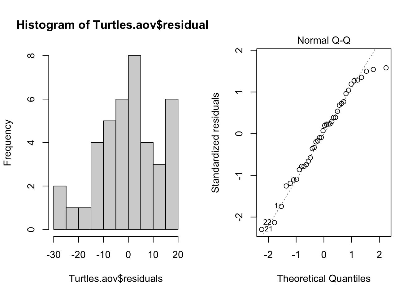
Violations of normality can be fixed via transformations or by using a different error-distribution in a generalised linear model (GLM).
Homogeneity of variance. The assumption of homgeneity of variance, namely that the variation in the residuals is approximately equal across the range of the predictor variable, can be checked by plotting the residuals against the fitted values from the aov model object.
plot(Turtles.aov, which = 1)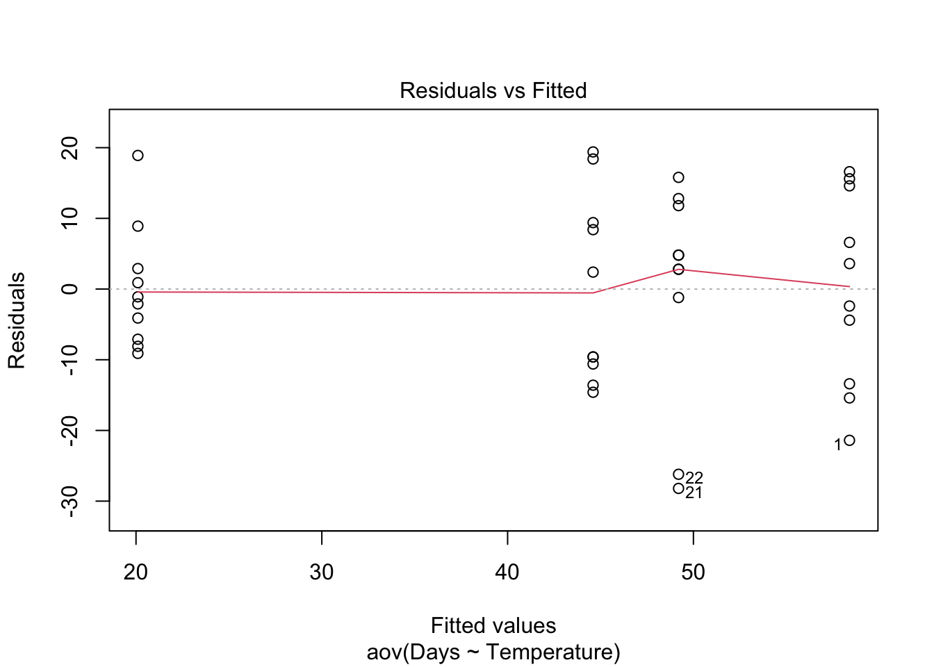
Heterogenous variances are indicated by non-random pattern in the residuals vs. fitted plot. Look for an even spread of the residuals on the y axis for each of the levels on the x axis. A fan-shaped distribution with more variance at higher values on the x axis is a common problem when data are skewed. See the testing assumptions of linear models module for more information. If there are strong patterns, one potential solution is to transform the response variable y. If this doesn’t fix the problem the best solution is to use a different error distribution in a generalised linear model (GLM).
Independence. ANOVA assumes that all replicate measures are independent of each other (i.e., equally likely to be sampled from the population of possible values for each level). This issue needs to be considered at the design stage. If data are grouped in any way (e.g., half the turtle eggs measured at one time, then the other half measured later), then more complex designs are needed to account for additional factors (e.g., a design with both temperature and time as factors).
There are a variety of measures for dealing with non-independence. These include ensuring all important predictors are in the model; averaging across nested observations; or using a mixed-model.
Communicating the results
Written. The results of a one-way ANOVA are usually expressed in text as a short sentence, e.g., “Turtle hatching time differed among the four incubation temperatures (F = 15.98, df = 3,36, p < 0.001)”. A significant effect would be followed by a written description of the post-hoc test results (i.e., exactly which temperatures differed from which). The results from post-hoc tests can also be added to the figure (e.g, by labelling which levels differed).
Visual. A boxplot or column graph with error bars are suitable for contrasting a continuous variable across levels of categorical variable. See the graphics help for making publication ready versions of these figures.
boxplot(Days ~ Temperature, data = Turtles, ylab = "Hatching time (days)", xlab = "Temperature (°C)")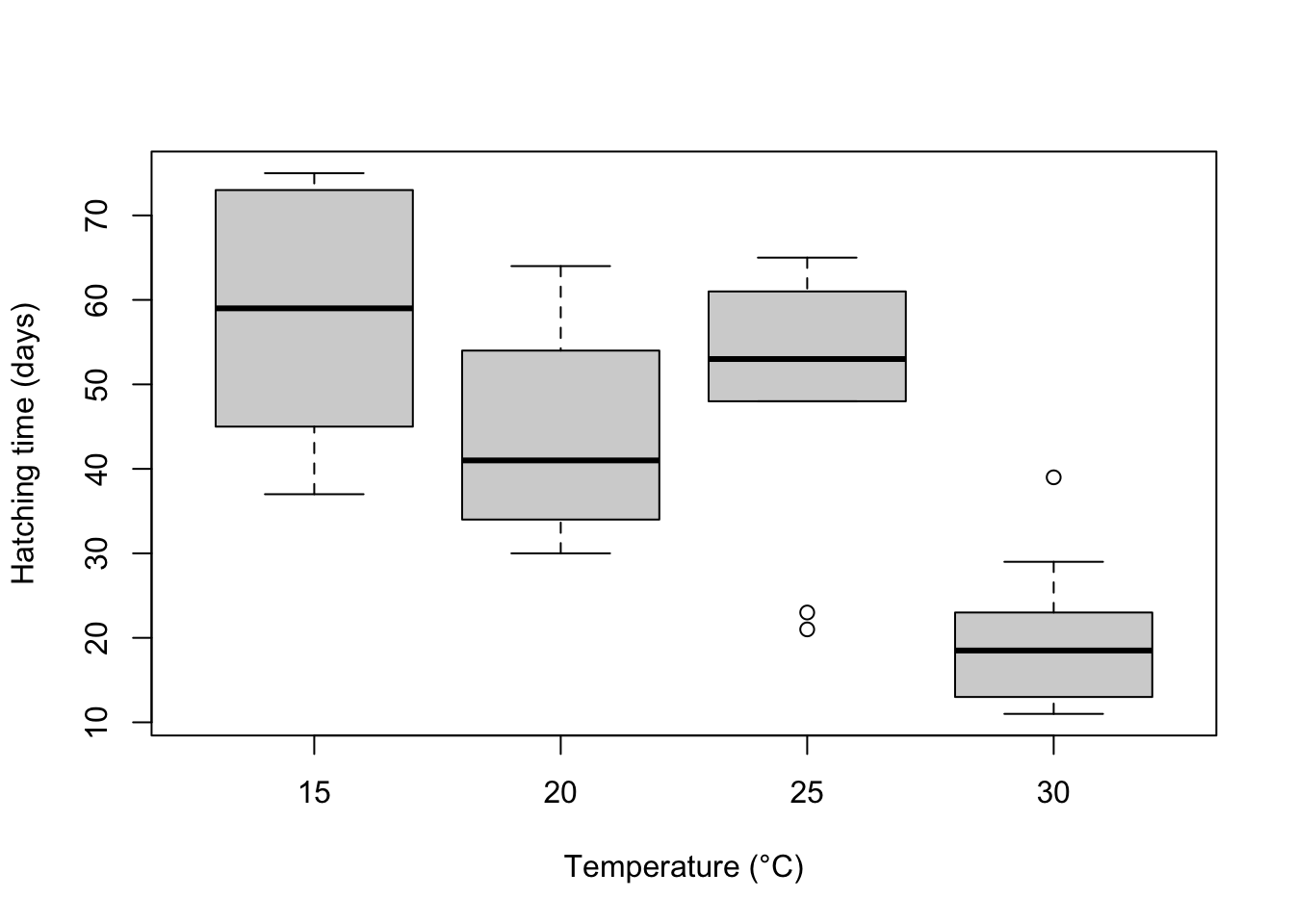
Further help
Type ?aov or ?lm to get the R help for these functions.
Quinn and Keough (2002) Experimental design and data analysis for biologists. Cambridge University Press. Ch. 8 Comparing groups or treatments - analysis of variance.
McKillup (2012) Statistics explained. An introductory guide for life scientists Cambridge University Press. Ch. 11. Single-factor analysis of variance.
Underood, AJ (1997) Experiments in ecology: Their logical design and interpretation using analysis of variance. Cambridge University Press.
Author: James Lavender
Year: 2016
Last updated: Feb 2022