Power Analyses
What is power analysis and why is it important?
You collect data to answer a question, usually with the aim of detecting a particular effect (e.g., treatment effect). The power of your test is the probability of detecting an effect (i.e., getting a p-value < 0.05) with the experimental design you have and the effect size that you expect or consider meaningful.
I’ll start by simulating a dataset which has an effect (a difference between the control and treatment), and we’ll see if we can detect the effect. We’ll do a simple two sample t-test for illustration.
set.seed(1)

N <- 20 # the sample size

trt.effect <- 0.2 # difference between control and treatment means
sigma <- 0.5 # standard deviation of control and treatment groups

mean.con <- 0 # mean of control group

mean.trt <- mean.con + trt.effect # mean of treatment group

control <- rnorm(N, mean.con, sigma) # 20 data points for the control group taken from a normal distribution with known sample size, mean and s.d.

treatment <- rnorm(N, mean.trt, sigma) # data for the treatment group

t.test(control, treatment)
##
## Welch Two Sample t-test
##
## data: control and treatment
## t = -0.71923, df = 37.917, p-value = 0.4764
## alternative hypothesis: true difference in means is not equal to 0
## 95 percent confidence interval:
## -0.3872163 0.1842117
## sample estimates:
## mean of x mean of y
## 0.09526194 0.19676424We can view the differences between the groups with a boxplot and test for those differences with a t-test:
boxplot(cbind(control, treatment))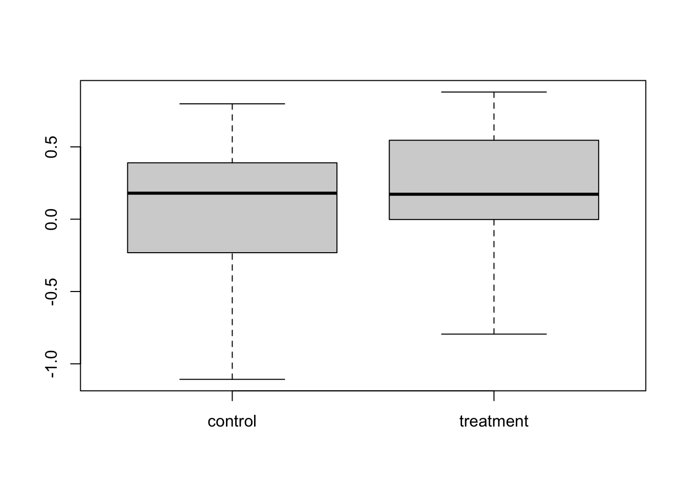
t.test(control, treatment)##
## Welch Two Sample t-test
##
## data: control and treatment
## t = -0.71923, df = 37.917, p-value = 0.4764
## alternative hypothesis: true difference in means is not equal to 0
## 95 percent confidence interval:
## -0.3872163 0.1842117
## sample estimates:
## mean of x mean of y
## 0.09526194 0.19676424We know there is an effect of treatment, with effect size 0.2, but the test was not able to detect it.This is known as a type II error. Let’s redo the same experiment with exactly the same setup.
#
set.seed(3)
N <- 20
trt.effect <- 0.2
sigma <- 0.5
mean.con <- 0
mean.trt <- mean.con + trt.effect
control <- rnorm(N, mean.con, sigma)
treatment <- rnorm(N, mean.trt, sigma)
boxplot(cbind(control, treatment))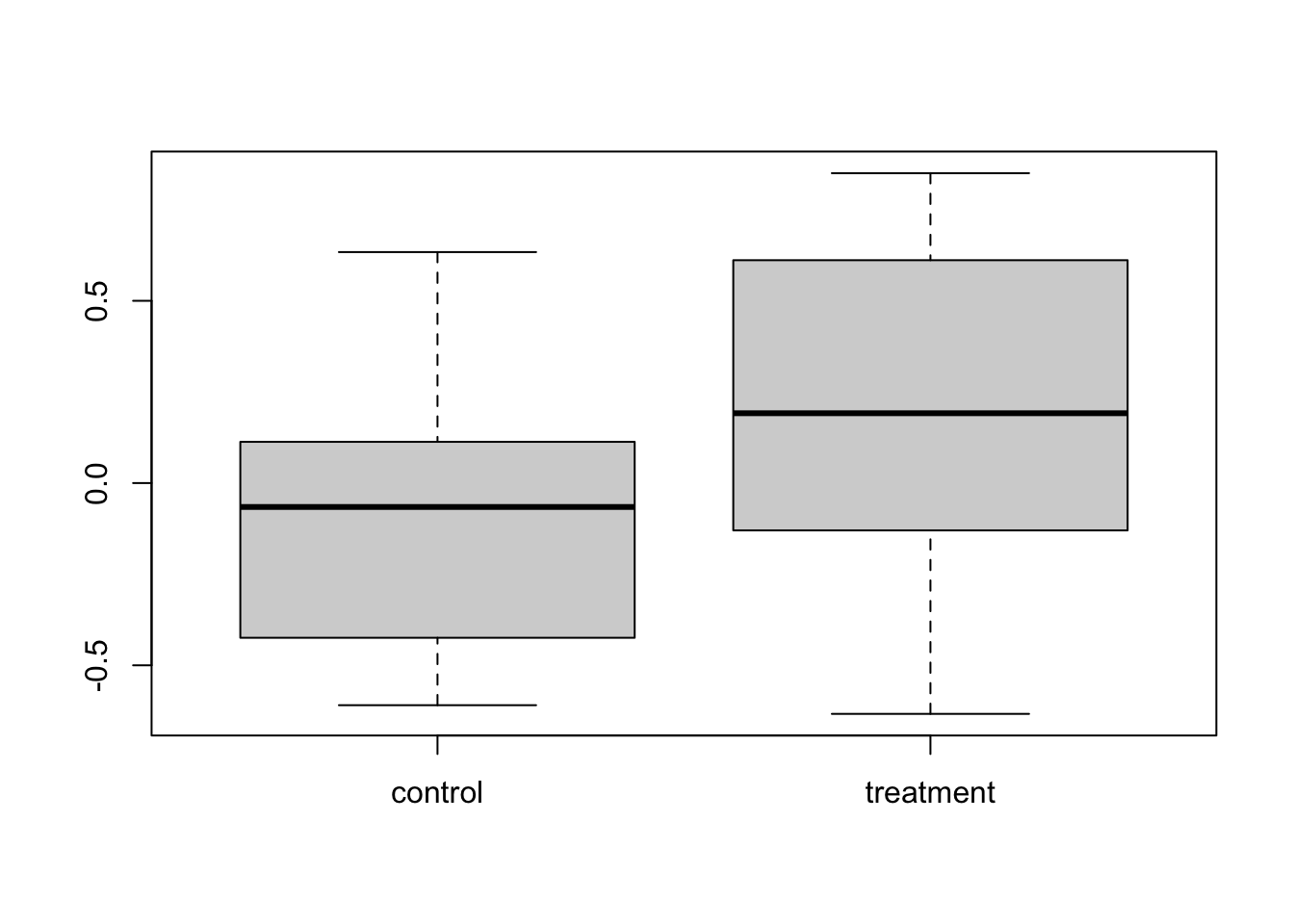
t.test(control, treatment)##
## Welch Two Sample t-test
##
## data: control and treatment
## t = -2.3471, df = 37.416, p-value = 0.02432
## alternative hypothesis: true difference in means is not equal to 0
## 95 percent confidence interval:
## -0.57817515 -0.04253493
## sample estimates:
## mean of x mean of y
## -0.08359522 0.22675982This time we did detect an effect. This always happens, no matter what your experimental design, if an effect is present, you have some chance of detecting it, this is called power. So as not to waste time and money, we should only conduct experiments that have high power, i.e. high probability of detecting an effect if there is one. We can calculate the power of this experiment.
Simple power analysis with ‘pwr’
There are various packages which do power analysis in R. pwr does simple stuff up to lm and simR does more complex mixed models and glms.
First, download and install the package.
library(pwr)To do power calculations in pwr, you leave one of the values as NULL and enter all the others. It then gives you the value for the one you left out.
Here I will use the function pwr.t.test and leave out power. It will calculate the power for the experimental design givne the specified sample size and effect size. Be careful; the d variable, which in the help file is called the effect size, is our treatment effect (difference between means) divided by the standard deviation.
pwr.t.test(n = 20, d = trt.effect / sigma, sig.level = 0.05, power = NULL)##
## Two-sample t test power calculation
##
## n = 20
## d = 0.4
## sig.level = 0.05
## power = 0.2343494
## alternative = two.sided
##
## NOTE: n is number in *each* groupWhoops, power is only about 25%. This means that given the effect we expect, and with this sample size, we will only detect that effect 25% of the time. So, it’s probably not worth doing this experiment. We could increase the sample size to increase power.
We can now use our power calculations to find out what sample size will give us good power, where 80% is the usual cutoff. We redo the calculation but now with N left blank and power = 0.8.
pwr.t.test(n = NULL, d = trt.effect / sigma, sig.level = 0.05, power = 0.8)##
## Two-sample t test power calculation
##
## n = 99.08032
## d = 0.4
## sig.level = 0.05
## power = 0.8
## alternative = two.sided
##
## NOTE: n is number in *each* groupThis tells us that to we need a sample size (for each group) of 100 to achieve 80% power of detecting our effect. This is obviously important to know if replicate measures are expensive or time consuming to collect.
We can also plot power for various sample sizes. Here is some code that calculates and plots power for samples sizes from 2 to 200.
nvals <- seq(2, 200, length.out = 200)
powvals <- sapply(nvals, function(x) pwr.2p.test(h = trt.effect / sigma, n = x, sig.level = 0.05)$power)

plot(nvals, powvals,
  xlab = "sample size", ylab = "power",
  main = "Power curve for sample size for difference in proportions",
  lwd = 2, col = "red", type = "l"
)

abline(h = 0.8)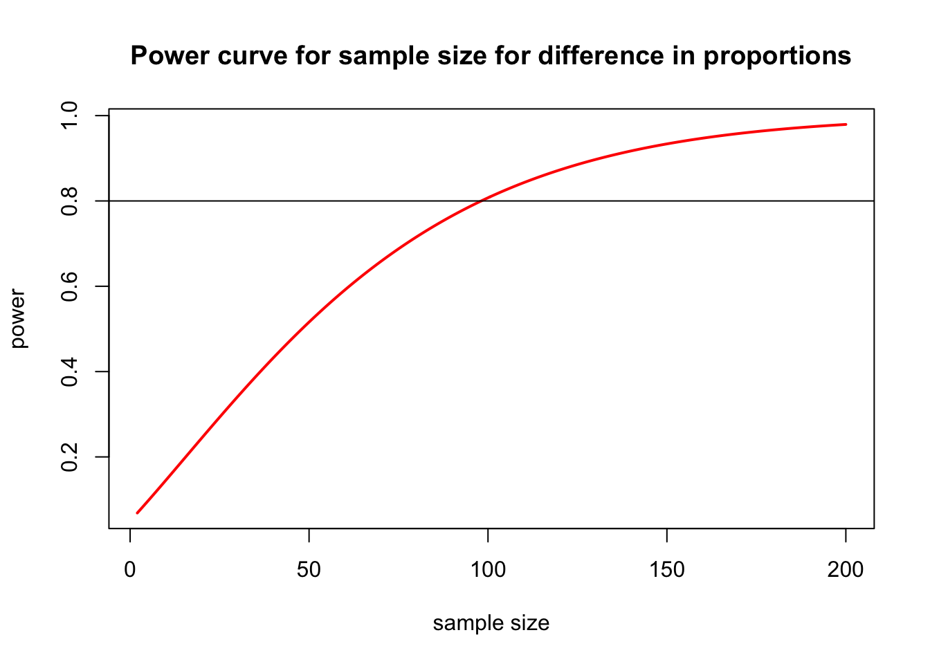
The pwr package has a bunch of functions, but they all pretty much work the same way.
| Function | Description |
|---|---|
pwr.2p.test |
two proportions (equal n) |
pwr.2p2n.test |
two proportions (unequal n) |
pwr.anova.test |
balanced one way ANOVA |
pwr.chisq.test |
chi-square test |
pwr.f2.test |
general linear model |
pwr.p.test |
proportion (one sample) |
pwr.r.test |
correlation |
pwr.t.test |
t-tests (one sample, 2 sample, paired) |
pwr.t2n.test |
t-test (two samples with unequal n) |
It is generally a bit tricky to specify effect size, you can find a good guide for this package here.
Note that specifying effect size is not a statistical question, it’s an ecological question of what effect size is meaningful for your particular study? For example, do you want to be able to detect a 10% decline in the abundance of a rare animal or would you be happy with a sampling design able to detect a 25% decline?
Analysis with linear and mixed models with ‘simr’
If you are conducting an experiment with random factors, and you need to do a mixed model and your power analysis needs to reflect that. This is much harder to do than the above examples, and we will need to use simulation methods. The package simR is designed to do this.
Download and install the package.
library(simr)
simrOptions(progress = FALSE)
Power analysis with a pilot study. We have conducted a pilot study, and now want to decide how we should allocate sampling for the full study. The study is looking for an effect of estuary modification on the abundance of a marine species. Let’s assume we have the resources to do a maximum of 72 samples, and we want to maximize power for a test of the categorical variable ‘modification’.

We have a pilot dataset ‘pilot’ which has a continuous fixed effect of temperature, a fixed effect of modification and a random effect for site (nested within modification). The response variable is the abundance of a species of interest.
Download this pilot data, Pilot.csv, import into R and change the modification variable into a factor (labelled as 1,2 and 3, but not an integer).
Pilot <- read.csv(file = "Pilot.csv", header = TRUE)
Pilot$modification <- factor(Pilot$modification)
Plotting abundance against site and the levels of the modification factor tells us that we have data where sites are quite variable within modification.
par(mfrow = c(1, 2))
boxplot(abundance ~ modification, data = Pilot, main = "modification")
boxplot(abundance ~ site, data = Pilot, main = "site")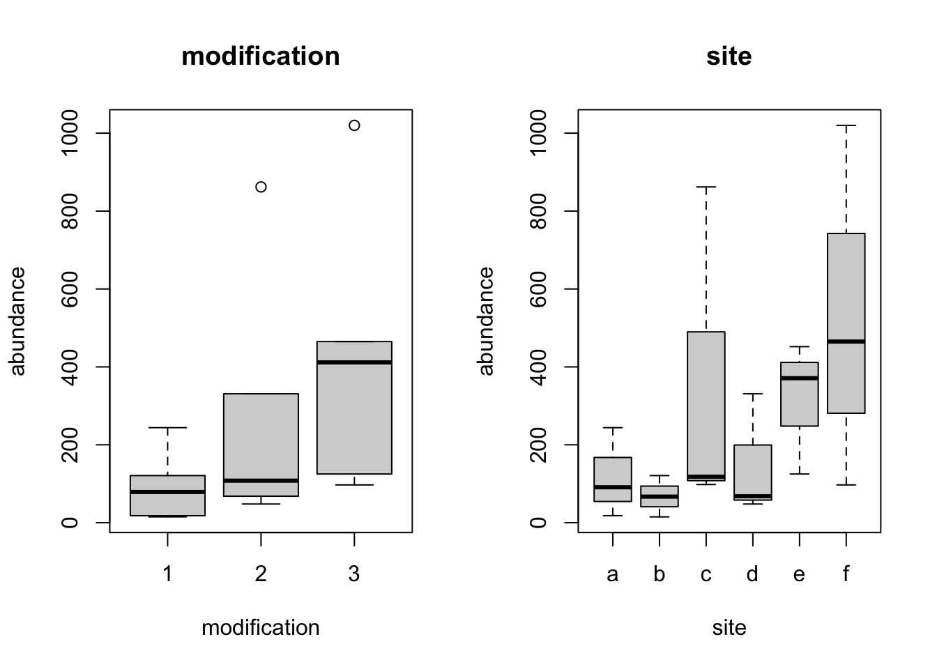
These count data with a random effect of site are best modelled with a generalised linear mixed model using glmer from the package lme4.
library(lme4)

Pilot.mod <- glmer(abundance ~ temperature + modification + (1 | site), family = "poisson", data = Pilot)

summary(Pilot.mod)
## Generalized linear mixed model fit by maximum likelihood (Laplace
## Approximation) [glmerMod]
## Family: poisson ( log )
## Formula: abundance ~ temperature + modification + (1 | site)
## Data: Pilot
##
## AIC BIC logLik deviance df.resid
## 153.3 157.7 -71.6 143.3 13
##
## Scaled residuals:
## Min 1Q Median 3Q Max
## -1.2983 -0.4266 0.1293 0.4240 0.8410
##
## Random effects:
## Groups Name Variance Std.Dev.
## site (Intercept) 0.006274 0.07921
## Number of obs: 18, groups: site, 6
##
## Fixed effects:
## Estimate Std. Error z value Pr(>|z|)
## (Intercept) 1.69024 0.09851 17.16 <2e-16 ***
## temperature 4.08409 0.08875 46.02 <2e-16 ***
## modification2 1.14103 0.09465 12.05 <2e-16 ***
## modification3 2.39503 0.09538 25.11 <2e-16 ***
## ---
## Signif. codes: 0 '***' 0.001 '**' 0.01 '*' 0.05 '.' 0.1 ' ' 1
##
## Correlation of Fixed Effects:
## (Intr) tmprtr mdfct2
## temperature -0.692
## modificatn2 -0.558 0.023
## modificatn3 -0.696 0.226 0.565There are two coefficients which specify effects of modification (as there are three modification categories). To do power analysis, we need to specify effect sizes for these which are ecologically meaningful. Keep in mind these are on the scale of the model, for a poisson model they are on the log scale (and multiplicative).
fixef(Pilot.mod)["modification2"] <- 0.1
fixef(Pilot.mod)["modification3"] <- 0.2
We can now use the powerSim function to calculate the probability of an experiment with this sample size being able to detect a this modification effect, this is the ‘power’. I want to use a likelihood ratio test (i.e., use the anova function) to test for an effect of modification, so I specify that with the lr argument.
powerSim(Pilot.mod, fixed("modification", "lr"), nsim = 50)## boundary (singular) fit: see ?isSingular
## boundary (singular) fit: see ?isSingular
## boundary (singular) fit: see ?isSingular
## boundary (singular) fit: see ?isSingular
## boundary (singular) fit: see ?isSingular
## boundary (singular) fit: see ?isSingular
## boundary (singular) fit: see ?isSingular
## boundary (singular) fit: see ?isSingular
## boundary (singular) fit: see ?isSingular
## boundary (singular) fit: see ?isSingular
## boundary (singular) fit: see ?isSingular
## boundary (singular) fit: see ?isSingular
## boundary (singular) fit: see ?isSingular
## boundary (singular) fit: see ?isSingular
## boundary (singular) fit: see ?isSingular
## boundary (singular) fit: see ?isSingular
## boundary (singular) fit: see ?isSingular
## boundary (singular) fit: see ?isSingular
## boundary (singular) fit: see ?isSingular
## boundary (singular) fit: see ?isSingular
## boundary (singular) fit: see ?isSingular
## boundary (singular) fit: see ?isSingular
## boundary (singular) fit: see ?isSingular
## boundary (singular) fit: see ?isSingular
## boundary (singular) fit: see ?isSingular
## boundary (singular) fit: see ?isSingular
## boundary (singular) fit: see ?isSingular
## boundary (singular) fit: see ?isSingular
## boundary (singular) fit: see ?isSingular
## boundary (singular) fit: see ?isSingular
## boundary (singular) fit: see ?isSingular
## boundary (singular) fit: see ?isSingular
## boundary (singular) fit: see ?isSingular
## boundary (singular) fit: see ?isSingular
## boundary (singular) fit: see ?isSingular
## boundary (singular) fit: see ?isSingular
## boundary (singular) fit: see ?isSingular
## boundary (singular) fit: see ?isSingular
## boundary (singular) fit: see ?isSingular
## boundary (singular) fit: see ?isSingular
## boundary (singular) fit: see ?isSingular## Power for predictor 'modification', (95% confidence interval):
## 46.00% (31.81, 60.68)
##
## Test: Likelihood ratio
##
## Based on 50 simulations, (0 warnings, 0 errors)
## alpha = 0.05, nrow = 18
##
## Time elapsed: 0 h 0 m 5 s# this is a small number of sims for demonstration, the default of 1000 is more appropriateSo we expect power of around 45% for a likelihood ratio test for ‘modification’ with the current number of observations. This is quite low, we would like to see power above 80%, so let’s see how increasing sample size affects that.
How can we increase power? Increasing observations is desirable to increase power, but in this sampling design, we have several ways of adding observations to your data. You could sample more sites, but keep the number of samples per site the same, or you could keep the number of sites the same, and sample more within each site.
xtabs(~ modification + site, data = Pilot)## site
## modification a b c d e f
## 1 3 3 0 0 0 0
## 2 0 0 3 3 0 0
## 3 0 0 0 0 3 3There are currently 2 sites per modification category and 3 observations per site. Let’s try to increase the number of sites. We do this by using the extend function to explore how increasing sample size will affect power. By using along=site, we will be adding further sites. With our budget of 72 observations and 3 observations per site, we would have 24 sites.
full1 <- extend(Pilot.mod, along = "site", n = 24)

xtabs(~site, data = attributes(full1)$newData)
## site
## 1 10 11 12 13 14 15 16 17 18 19 2 20 21 22 23 24 3 4 5 6 7 8 9
## 3 3 3 3 3 3 3 3 3 3 3 3 3 3 3 3 3 3 3 3 3 3 3 3powerSim(full1, fixed("modification", "lr"), nsim = 50)## boundary (singular) fit: see ?isSingular
## boundary (singular) fit: see ?isSingular## Power for predictor 'modification', (95% confidence interval):
## 92.00% (80.77, 97.78)
##
## Test: Likelihood ratio
##
## Based on 50 simulations, (0 warnings, 0 errors)
## alpha = 0.05, nrow = 72
##
## Time elapsed: 0 h 0 m 5 sSo we get about 90% power, sounds great. To see whether adding more observations per site would do better or worse, for use the within argument.
full2 <- extend(Pilot.mod, within = "site", n = 12)
xtabs(~site, data = attributes(full2)$newData)## site
## a b c d e f
## 12 12 12 12 12 12powerSim(full2, fixed("modification", "lr"), nsim = 50)## boundary (singular) fit: see ?isSingular
## boundary (singular) fit: see ?isSingular
## boundary (singular) fit: see ?isSingular
## boundary (singular) fit: see ?isSingular
## boundary (singular) fit: see ?isSingular
## boundary (singular) fit: see ?isSingular
## boundary (singular) fit: see ?isSingular
## boundary (singular) fit: see ?isSingular
## boundary (singular) fit: see ?isSingular
## boundary (singular) fit: see ?isSingular
## boundary (singular) fit: see ?isSingular
## boundary (singular) fit: see ?isSingular## Power for predictor 'modification', (95% confidence interval):
## 64.00% (49.19, 77.08)
##
## Test: Likelihood ratio
##
## Based on 50 simulations, (0 warnings, 0 errors)
## alpha = 0.05, nrow = 72
##
## Time elapsed: 0 h 0 m 5 sThat only gives us about 60% power. So for this data, sampling design and question, it is better to add more sites. Of course you can also do combinations, maybe double the sites and double the observations per site.
full3 <- extend(Pilot.mod, within = "site", n = 6)
full3 <- extend(full3, along = "site", n = 12)

xtabs(~site, data = attributes(full3)$newData)
## site
## 1 10 11 12 2 3 4 5 6 7 8 9
## 6 6 6 6 6 6 6 6 6 6 6 6powerSim(full3, fixed("modification", "lr"), nsim = 50)## boundary (singular) fit: see ?isSingular
## boundary (singular) fit: see ?isSingular
## boundary (singular) fit: see ?isSingular
## boundary (singular) fit: see ?isSingular
## boundary (singular) fit: see ?isSingular
## boundary (singular) fit: see ?isSingular## Power for predictor 'modification', (95% confidence interval):
## 66.00% (51.23, 78.79)
##
## Test: Likelihood ratio
##
## Based on 50 simulations, (0 warnings, 0 errors)
## alpha = 0.05, nrow = 72
##
## Time elapsed: 0 h 0 m 5 sThis gives 75% power, which is midway between the others. So in this case it is again better to add more sites than more observations per site. This is by no means always true, and depended to a large extent on the variability within and between sites, your experimental design, your question.
Some notes
Power analysis give the probability of detecting a particular effect (of a particular strength), at a particular alpha level (usually 0.05) if this effect is present. If you are interested in multiple questions from the same data, to do power analysis you generally have to chose a question of primary interest.
You need to specify the level of the effect that you want to be able to detect, if you use the estimated level from a pilot study, this is called an “observed power” calculation, and is not a valid use of power analysis.
Further information
Some more examples from pilot studies from the simR package
Power analysis from scratch with no pilot study
More on specifying effect size
Author: Gordana Popovic
Year: 2016
Last updated: Feb 2022