Multivariate Analysis with mvabund
Multivariate data are common in the environmental sciences, occurring when ever we measure several response variables from each replicate sample. Questions like how does the species composition of a community vary across sites, or how does the shape of trees (as measured by several morphological traits) vary with altitude are multivariate questions.
We will use the package mvabund to specify and fit multivariate statistical models to these sorts of data.
How does this method differ from other multivariate analyses? Many commonly used analyses for multivariate data sets (e.g. PERMANOVA, ANOSIM, CCA, RDA etc.) are “distance-based analyses”. This means the first step of the analysis is to calculate a measure of similarity between each pair of samples, thus converting a multivariate dataset into a univariate one.
There are a couple of problems with these kinds of analysis. First, their statistical power is very low, except for variables with high variance. This means that for variables which are less variable, the analyses are less likely to detect a treatment effect. Second, they do not account for a very important property of multivariate data, which is the mean-variance relationship. Typically, in multivariate datasets like species-abundance data sets, counts for rare species will have many zeros with little variance, and the higher counts for more abundant species will be more variable.
The mvabund approach improves power across a range of species with different variances and includes an assumption of a mean-variance relationship. It does this by fitting a single generalised linear model (GLM) to each response variable with a common set of predictor variables. We can then use resampling to test for significant community level or species level responses to our predictors.
Also, the model-based framework makes it easier to check our assumptions and interpret uncertainty around our findings.
If you’re interested in this method, watch the introductory video, Introducing mvabund and why multivariate statistics in ecology is a bit like Rick Astley…

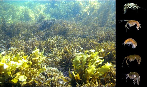
In this example, we use a data set where researchers wanted to contrast the species composition of marine herbivores on five species of macroalgae. Twenty replicate individuals of each of seven species of macroalgae were collected from Sydney Harbour, and the abundance of seven species of herbivorous crustacean recorded from each replicate (data from Poore et al. 2000). The data are multivariate because seven response variables (the species) were measured from each of the samples.
We could reduce this into a univariate dataset by calculating the 4950 (100*99/2) pairwise differences between samples, and use these differences to visualise patterns in the data (e.g, as we did in our multi-dimensional scaling example) or test hypotheses about groups of samples by resampling these differences.
Here, we will use mvabund to contrast species composition across habitats using models that are appropriate for the mean-variance relationships and allowing us to check assumptions of those models.
Running the analysis
First, install and load the mvabund package.
library(mvabund)Your data should be formatted so that each sample is a row and each variable is a column. Download the herbivore specialisation data set, and import into R to see the desired format.
Herbivores <- read.csv(file = "Herbivore_specialisation.csv", header = TRUE)The first two columns are categorical variables that label the samples as coming from each of the five habitats or as being collected during the day or the night. The third column is the replicate number per combination of habitat and day/night. The fourth column is the biomass of the habitat sampled and the rest of the columns are the counts of each herbivore species in each sample.
We will now use the just the abundance data (in columns 5 to 11) and convert it to an mvabund object format used by the mvabund package.
Herb_spp <- mvabund(Herbivores[, 5:11])We can have a quick look at the spread of our data using the boxplot function.
par(mar = c(2, 10, 2, 2)) # adjusts the margins
boxplot(Herbivores[, 5:11], horizontal = TRUE, las = 2, main = "Abundance")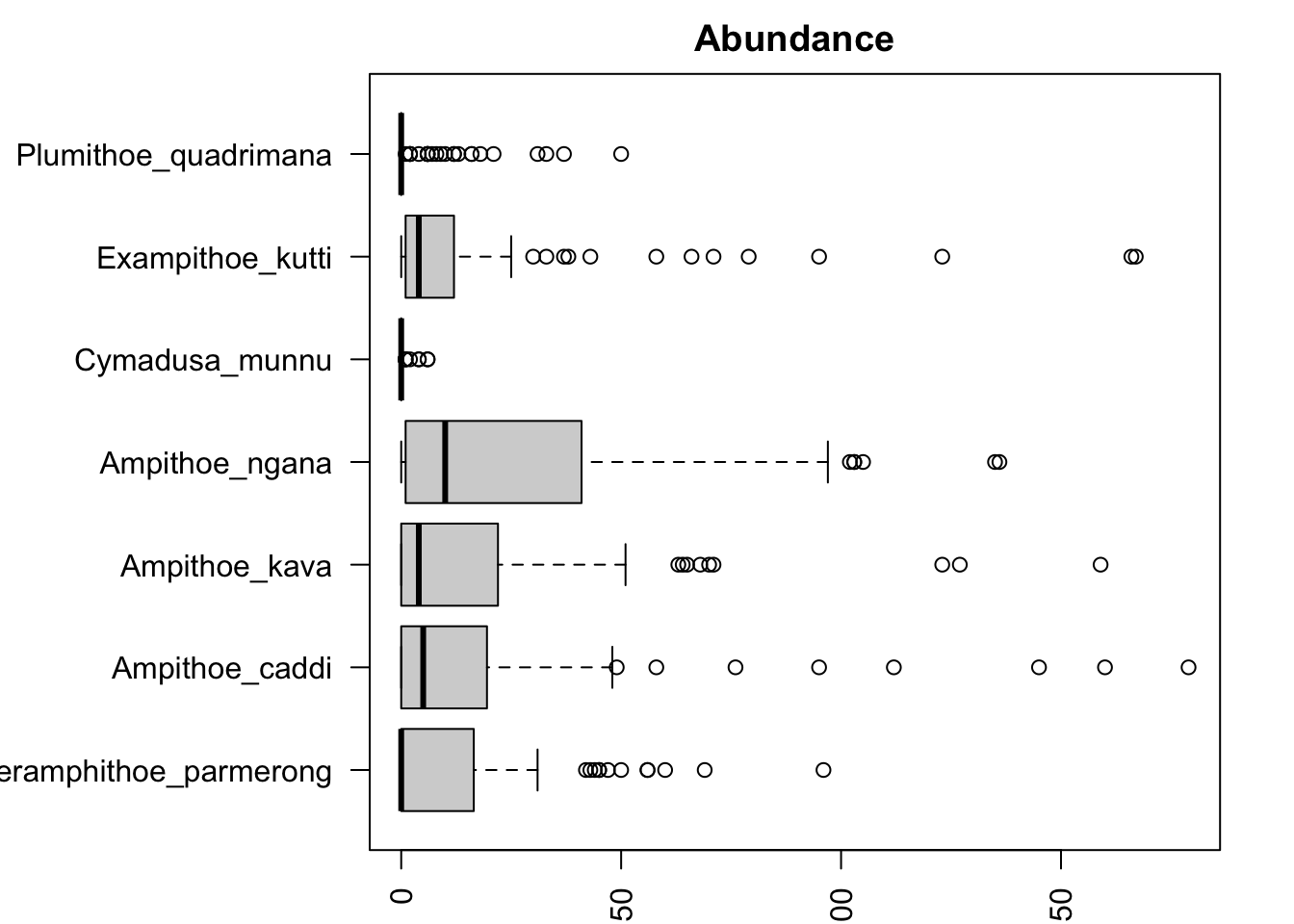
It looks like some species of marine herbivores (e.g. Ampithoe ngana) are much more abundant and variable than others (e.g. Cymadusa munnu). It’s probably a good idea to check our mean-variance relationship then! We can do this using the meanvar.plot function:
meanvar.plot(Herb_spp)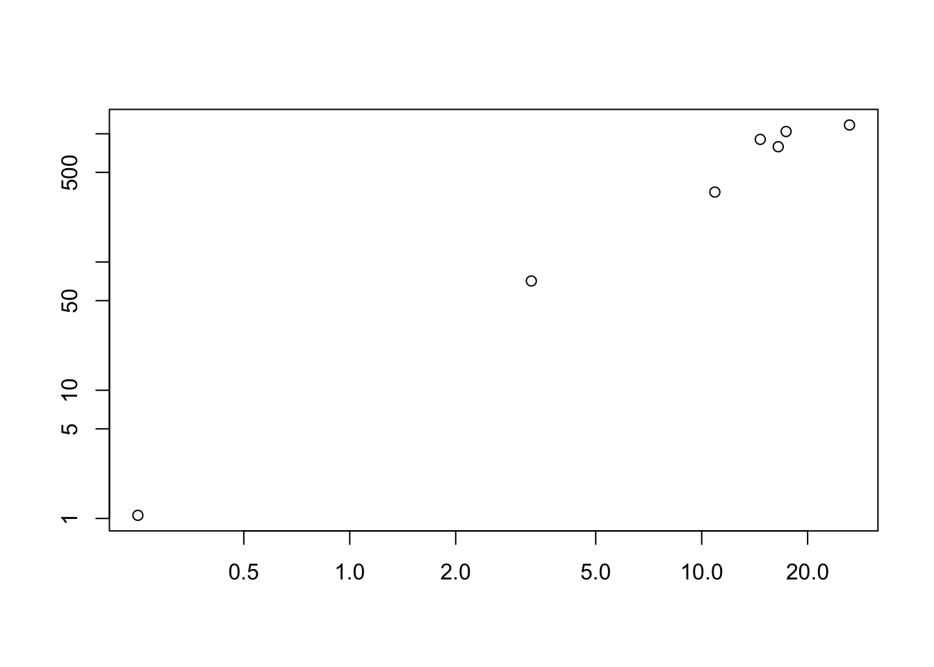
You can clearly see that the species with high means (on the x axis) also have high variances (y axis).
We can deal with this relationship by choosing a family of GLMs with an appropriate mean-variance assumption. The default family used by mvabund when fitting multivariate GLMs is negative binomial which assumes a quadratic mean-variance relationship and a log-linear relationship between the response variables and any continuous variables. In this example, we only have categorical variables so that one’s not too important. If you are unsure of these relationships, don’t worry, we can check our model fit later.
Now let’s get back to our research questions. Are there differences in the species composition of the seven marine herbivores sampled? Do some of them specialise on particular types of algae while others are more generalised feeders? Which species? Let’s start by eyeballing the data.
There is a ‘quick and dirty’ built-in plotting function in the mvabund package that allows us to contrast transformed abundances to the predictor variables of our choice. To contrast abundances against habitat, we would use:
plot(Herb_spp ~ as.factor(Herbivores$Habitat), cex.axis = 0.8, cex = 0.8)##
## PIPING TO 2nd MVFACTOR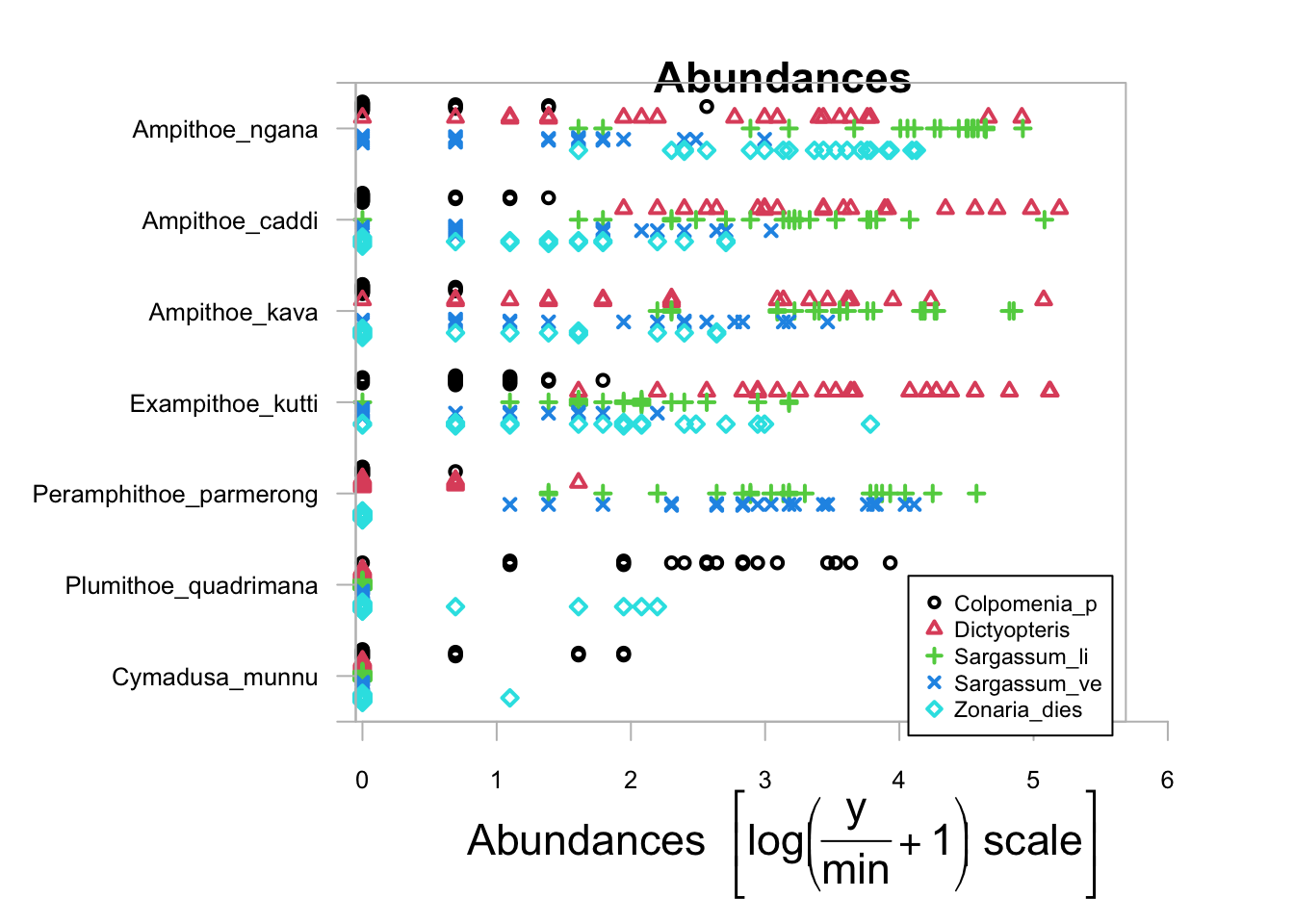
Alternatively, we can include the argument transformation="no" to look at the raw abundance data. Because this plot is based on the base plotting language in R, you can add extra arguments to customise the graph. We have made the axis text (cex.axis=0.8) and the symbols (cex=0.8) smaller so that we can better see what’s going on.
It is quite a messy graph but a couple of things jump out at us. It looks like the herbivore Ampithoe ngana is very abundant and will eat just about anything. On the other hand, Cymadusa munnu and Plumithoe quadrimana are quite rare. Ampithoe ngana, A. caddi, A. kava and Exampithoe kutti are generalist feeders whereas Perampithoe parmerong is largely specialised to the two species of Sargassum.
Let’s now contrast the species composition across algal species to see if the models support our observations.
The model syntax below fits our response variable (the mvabund object Herb_spp with the 100 counts of 7 species) to the predictor variable Habitat (type of algae).
mod1 <- manyglm(Herb_spp ~ Herbivores$Habitat, family = "poisson")Assumptions to check
Before we examine the output, we need to check our model assumptions. We can use the plot function to generate a plot of residuals.
plot(mod1)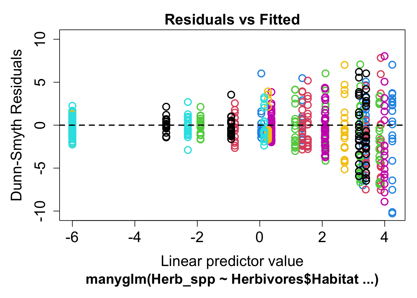
If the model is a good fit, we should see a random scatter of points. What we don’t want to see is a relationship, either linear or curvilinear, or a fan shape. This could mean that one of our assumptions was wrong: either our mean-variance relationship was wrongly specified, or our assumed relationship between our response and predictors was incorrect. Or, we could have missed a key explaining variable in our model which leaves a lot of unexplained variance.
In this example, we see a clear fan shape in the residual plot, this means we have misspecified our mean-variance relationship. We can use the family argument to choose a distribution which is better suited to our data. For count data which does not fit the 'poisson distribution, we can use the negative_binomial distribution.
mod2 <- manyglm(Herb_spp ~ Herbivores$Habitat, family = "negative_binomial")
plot(mod2)
## Warning in default.plot.manyglm(x, res.type = res.type, which = which, caption =
## caption, : Only the first 7 colors will be used for plotting.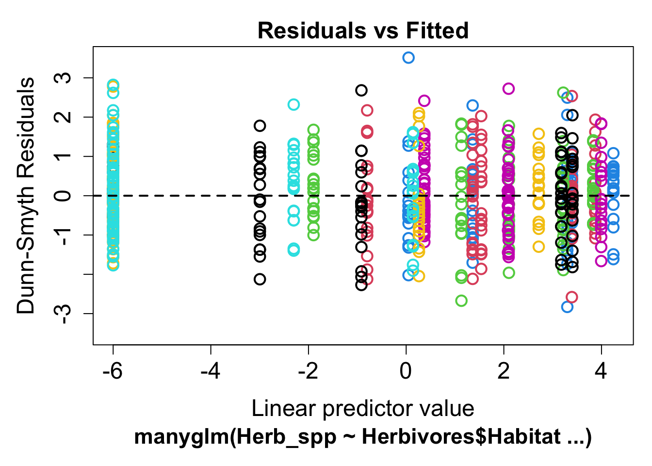
This residual plot is much better, there is now no discernible fan shape and we will use this model for all further analysis.
Interpreting the results
We can test the multivariate hypothesis of whether species composition varied across the habitats by using the anova function. This gives an analysis of deviance table where we use likelihood ratio tests and resampled p values to look for a significant effect of Habitat on the community data.
anova(mod2)## Time elapsed: 0 hr 0 min 7 sec## Analysis of Deviance Table
##
## Model: Herb_spp ~ Herbivores$Habitat
##
## Multivariate test:
## Res.Df Df.diff Dev Pr(>Dev)
## (Intercept) 99
## Herbivores$Habitat 95 4 625.2 0.001 ***
## ---
## Signif. codes: 0 '***' 0.001 '**' 0.01 '*' 0.05 '.' 0.1 ' ' 1
## Arguments:
## Test statistics calculated assuming uncorrelated response (for faster computation)
## P-value calculated using 999 iterations via PIT-trap resampling.We can see from this table that there is a significant effect of Habitat (LRT = 625, P = 0.001), meaning that the species composition of herbivores clearly differs between the species of algae that they are found on.
To examine this further, and see which herbivore species are more likely to be found on which algal species, we can run univariate tests for each species separately.
This is done by using the p.uni="adjusted" argument in the anova function. The “adjusted” part of the argument refers to the resampling method used to compute the p values, taking into account the correlation between the response variables. This correlation is often found in ecological systems where different species will interact with each other, competing with or facilitating each others’ resource use.
anova(mod2, p.uni = "adjusted")## Time elapsed: 0 hr 0 min 7 sec## Analysis of Deviance Table
##
## Model: Herb_spp ~ Herbivores$Habitat
##
## Multivariate test:
## Res.Df Df.diff Dev Pr(>Dev)
## (Intercept) 99
## Herbivores$Habitat 95 4 625.2 0.001 ***
## ---
## Signif. codes: 0 '***' 0.001 '**' 0.01 '*' 0.05 '.' 0.1 ' ' 1
##
## Univariate Tests:
## Peramphithoe_parmerong Ampithoe_caddi
## Dev Pr(>Dev) Dev Pr(>Dev)
## (Intercept)
## Herbivores$Habitat 148.716 0.001 91.659 0.001
## Ampithoe_kava Ampithoe_ngana
## Dev Pr(>Dev) Dev Pr(>Dev)
## (Intercept)
## Herbivores$Habitat 85.366 0.001 90.221 0.001
## Cymadusa_munnu Exampithoe_kutti
## Dev Pr(>Dev) Dev Pr(>Dev)
## (Intercept)
## Herbivores$Habitat 21.452 0.001 107.254 0.001
## Plumithoe_quadrimana
## Dev Pr(>Dev)
## (Intercept)
## Herbivores$Habitat 80.575 0.001
## Arguments:
## Test statistics calculated assuming uncorrelated response (for faster computation)
## P-value calculated using 999 iterations via PIT-trap resampling.Even after adjusting for multiple testing, there is an effect of habitat on all species.
So far, we have considered just one predictor variable of habitat. By altering the formula in mvabund, we can test more complex models. For example, to fit a model with both habitat and day or night, we would use:
mod3 <- manyglm(Herb_spp ~ Herbivores$Habitat * Herbivores$DayNight, family = "negative_binomial")
anova(mod3)
## Time elapsed: 0 hr 0 min 23 sec## Analysis of Deviance Table
##
## Model: Herb_spp ~ Herbivores$Habitat * Herbivores$DayNight
##
## Multivariate test:
## Res.Df Df.diff Dev Pr(>Dev)
## (Intercept) 99
## Herbivores$Habitat 95 4 625.2 0.001 ***
## Herbivores$DayNight 94 1 6.2 0.586
## Herbivores$Habitat:Herbivores$DayNight 90 4 25.4 0.449
## ---
## Signif. codes: 0 '***' 0.001 '**' 0.01 '*' 0.05 '.' 0.1 ' ' 1
## Arguments:
## Test statistics calculated assuming uncorrelated response (for faster computation)
## P-value calculated using 999 iterations via PIT-trap resampling.You can see that the species composition of herbivores varies with habitat, but not between day and night.
Communicating the results
Written. If we were writing a paper about the differences in habitat use by marine herbivores, we may write the following: There were different marine herbivores communities on different algal substrates (LRT = 625, P < 0.001). We can be more descriptive about the community differences by using a graphical representation of our results.
Visual. Multivariate data are best visualised by ordination plots. See the boral package for model based ordination. To get started, watch this video.
Further help
This method was created by UNSW’s Ecostats research group, you can keep up with their latest research on their blog. They have been updating the mvabund package with many new exciting features, including block resampling and fourth corner analyses.
Wang, Y, U Naumann, ST Wright & DI Warton (2012) mvabund - an R package for model-based analysis of multivariate abundance data. Methods in Ecology and Evolution 3: 471-474.
Authors: Rachel V. Blakey & Andrew Letten
Year: 2016
Last updated: Feb 2022