Crossed and Nested Factors
Mixed models 1 is an introduction to mixed models with one random factor. After reading that, if you think you have more than one random factor, then read on. For example, you might have crossed or nested factors.
Many experimental designs in ecology and environmental sciences require mixed models with several random effects (factors). You might have heard of nested and crossed factors. We often define these as quite distinct designs (e.g., from www.theanalysisfactor.com)
Two factors are crossed when every category (level) of one factor co-occurs in the design with every category of the other factor. In other words, there is at least one observation in every combination of categories for the two factors.
A factor is nested within another factor when each category of the first factor co-occurs with only one category of the other. In other words, an observation has to be within one category of Factor 2 in order to have a specific category of Factor 1. All combinations of categories are not represented.
There are also intermediate designs that are partially crossed, where some levels of one factor occur in several (but not all) levels of the second factor. These designs have often been taught as separate problems with different ways to carry out analyses of variance (ANOVAs) depending on if you have crossed or nested factors. Using mixed models with the package lme4, we can think if all of these in one framework, where nested and crossed designs are modelled in the same way. Thinking about factors as crossed or nested is simplified to careful labelling of factor levels - more on this later.
Running the analysis
We will use the package lme4 for all our mixed effect modelling. It will allow us to model both continuous and discrete data with one or more random effects. First, load the package:
library(lme4)We will analyse a data set that aimed to test the effect of water pollution on the abundance of some subtidal marine invertebrates by comparing samples from modified and pristine estuaries. As the total counts are large, we will assume the data are continuous. Later on, in Mixed models 3, we’ll model counts as discrete using Generalised linear mixed models (GLMMs).

Download the sample data set, Estuaries.csv, and load into R.
Estuaries <- read.csv("Estuaries.csv", header = T)Fitting a model with a fixed effect and several random effects
In this data set, we have a fixed effect (Modification; modified vs pristine) and two random effects (Estuary and Site). Site is nested within Estuary as each site can only belong in one estuary. When entering the data, however, we’ve been careless and numbered sites within each estuary as 1, 2, 3 etc.
We can see this by looking at the data, and a cross tabulation.
Estuaries[1:10, ]## X Modification Estuary Site Hydroid Total Schizoporella.errata
## 1 1 Modified JAK 1 0 44 15
## 2 2 Modified JAK 1 0 42 8
## 3 3 Modified JAK 2 0 32 9
## 4 4 Modified JAK 2 0 44 14
## 5 5 Modified JAK 3 1 42 6
## 6 6 Modified JAK 3 1 48 12
## 7 7 Modified JAK 4 0 45 28
## 8 8 Modified JAK 4 0 34 1
## 9 9 Pristine JER 1 7 29 0
## 10 10 Pristine JER 1 5 51 0xtabs(~ Estuary + Site, Estuaries, sparse = TRUE)## 7 x 4 sparse Matrix of class "dgCMatrix"
## Site
## Estuary 1 2 3 4
## BOT 2 2 2 2
## CLY 2 2 2 2
## HAK 2 2 2 2
## JAK 2 2 2 2
## JER 2 2 2 2
## KEM 2 2 . 2
## WAG 2 2 2 2Estuary JAK and estuary JER each have sites numbered 1, even though these sites are not connected in any way. We can also see this in the cross tabulation xtabs. This site labelling looks crossed, where each site occurs in each estuary, rather than nested.
We can fix this by simply telling R that Site is nested in Estuary. It is best practice, however, to do this at the data entry stage. If things are the same, then they should be labelled the same, and if they are not they should be labelled differently.
To create a unique label for each site in this data set, we convert Site to a factor (it was an integer), and create a new variable (SiteWithin) that is the combination of Estuary and Site
Estuaries$Site <- as.factor(Estuaries$Site)

Estuaries$SiteWithin <- paste0(Estuaries$Estuary, "_", Estuaries$Site)
Now, check the structure to see that each site is nested in only one Estuary, consistent with the experimental design.
xtabs(~ Estuary + SiteWithin, Estuaries, sparse = TRUE)## 7 x 27 sparse Matrix of class "dgCMatrix"## [[ suppressing 27 column names 'BOT_1', 'BOT_2', 'BOT_3' ... ]]##
## BOT 2 2 2 2 . . . . . . . . . . . . . . . . . . . . . . .
## CLY . . . . 2 2 2 2 . . . . . . . . . . . . . . . . . . .
## HAK . . . . . . . . 2 2 2 2 . . . . . . . . . . . . . . .
## JAK . . . . . . . . . . . . 2 2 2 2 . . . . . . . . . . .
## JER . . . . . . . . . . . . . . . . 2 2 2 2 . . . . . . .
## KEM . . . . . . . . . . . . . . . . . . . . 2 2 2 . . . .
## WAG . . . . . . . . . . . . . . . . . . . . . . . 2 2 2 2To fit a model for total abundance, we would use:
fit.mod <- lmer(Total ~ Modification + (1 | Estuary) + (1 | SiteWithin), data = Estuaries)
summary(fit.mod)
## Linear mixed model fit by REML ['lmerMod']
## Formula: Total ~ Modification + (1 | Estuary) + (1 | SiteWithin)
## Data: Estuaries
##
## REML criterion at convergence: 386.6
##
## Scaled residuals:
## Min 1Q Median 3Q Max
## -1.8686 -0.6687 0.1504 0.6505 1.9816
##
## Random effects:
## Groups Name Variance Std.Dev.
## SiteWithin (Intercept) 49.85 7.061
## Estuary (Intercept) 47.59 6.899
## Residual 43.65 6.607
## Number of obs: 54, groups: SiteWithin, 27; Estuary, 7
##
## Fixed effects:
## Estimate Std. Error t value
## (Intercept) 41.053 4.739 8.662
## ModificationPristine -14.553 6.232 -2.335
##
## Correlation of Fixed Effects:
## (Intr)
## MdfctnPrstn -0.760where Total is the dependent variable (left of the ~), Modification is the fixed effect, and Estuary and SiteWithin are the random effects.
We’ll also fit the wrong model, to see the difference if we had used the old labels for each site.
fit.wrong <- lmer(Total ~ Modification + (1 | Estuary) + (1 | Site), data = Estuaries)
summary(fit.wrong)
## Linear mixed model fit by REML ['lmerMod']
## Formula: Total ~ Modification + (1 | Estuary) + (1 | Site)
## Data: Estuaries
##
## REML criterion at convergence: 393.6
##
## Scaled residuals:
## Min 1Q Median 3Q Max
## -2.3312 -0.7631 0.1040 0.5766 1.8202
##
## Random effects:
## Groups Name Variance Std.Dev.
## Estuary (Intercept) 53.613 7.322
## Site (Intercept) 7.686 2.772
## Residual 80.045 8.947
## Number of obs: 54, groups: Estuary, 7; Site, 4
##
## Fixed effects:
## Estimate Std. Error t value
## (Intercept) 41.257 4.849 8.508
## ModificationPristine -14.757 6.124 -2.410
##
## Correlation of Fixed Effects:
## (Intr)
## MdfctnPrstn -0.727The only place we can see an obvious difference is under the Random effects table. For the correct model we have Number of obs: 52, groups: SiteWithin, 26; Estuary, 7 while the wrong model tells us we have only 4 sites, which we know is incorrect.
Note: fit.wrong would be correct if we had crossed factors
Checking assumptions
The assumptions are the same as for one random factor, but it doesn’t hurt to list them again
- The observed \(y\) are independent, conditional on some predictors \(x\)
- The response \(y\) are normally distributed conditional on some predictors \(x\)
- The response \(y\) has constant variance, conditional on some predictors \(x\)
- There is a straight line relationship between \(y\) and the predictors \(x\) and random effects \(z\)
- Random effects \(z\) are independent of \(y\).
- Random effects \(z\) are normally distributed
See Mixed models 1 for detailed guidance about assumptions in linear mixed models. Briefly, assumptions 1 and 5 cannot be checked, but can be ensured by taking random samples, and assumption 6 is not crucial and difficult to check. To check assumption 2 we look for a straight line relationship on the normal quantile plot. To check assumptions 3, and 4 we look for a fan shape and U shape on the residual vs. fitted plot.
par(mfrow = c(1, 2))
qqnorm(residuals(fit.mod))
scatter.smooth(residuals(fit.mod) ~ fitted(fit.mod)) # residual plot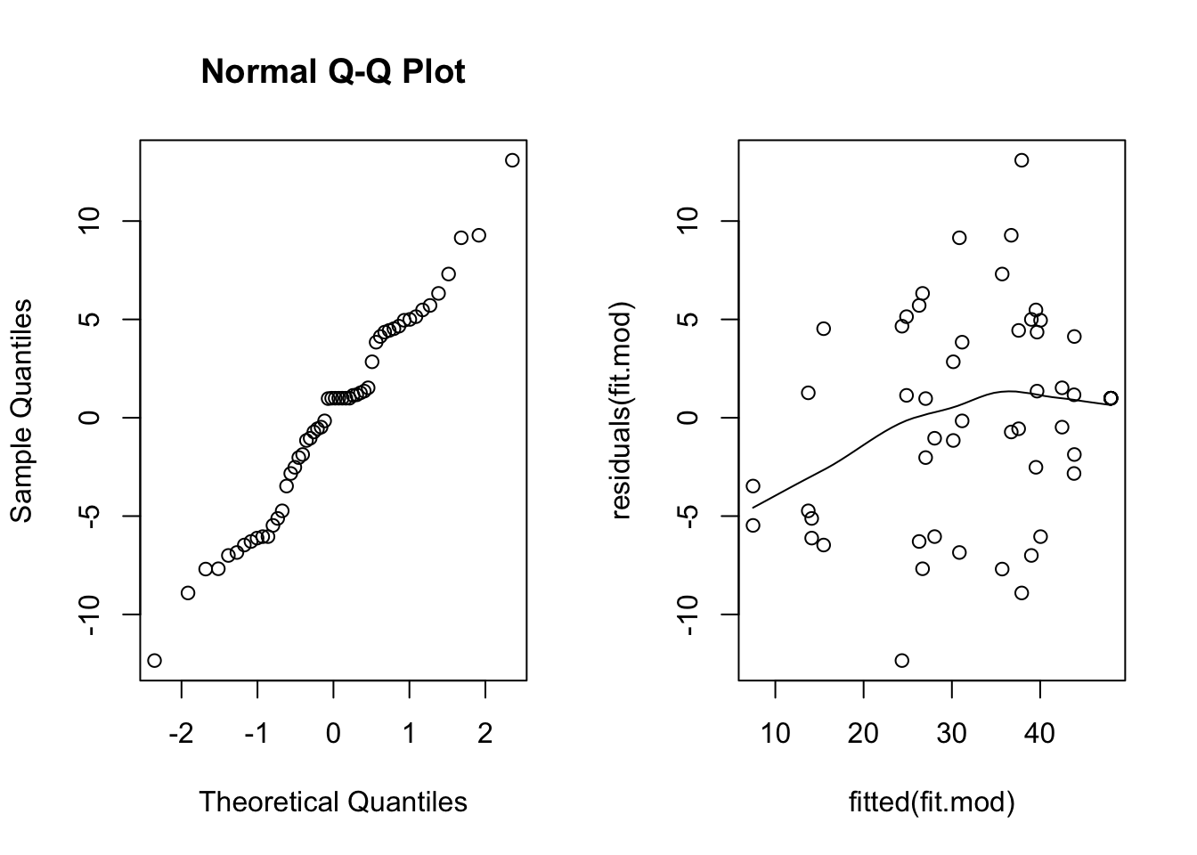
The normal quantile plot looks reasonable, however we see here a definite fan shape in the residual vs. fit plot. Let’s try transforming the response and see if we do better.
fit.mod <- lmer(log(Total) ~ Modification + (1 | Estuary) + (1 | SiteWithin), data = Estuaries)
par(mfrow = c(1, 2))
qqnorm(residuals(fit.mod))
scatter.smooth(residuals(fit.mod) ~ fitted(fit.mod)) # residual plot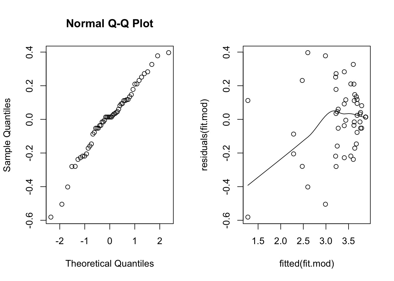
This scatterplot is much better, the fan shape is all but gone. The smooth line is below zero on the left, but there are relatively few points there, so it’s not of great concern.
Interpreting the results
Hypothesis test for the fixed effect
We can use the anova as before to obtain approximate p-values for fixed effects.
ft.mod <- lmer(log(Total) ~ Modification + (1 | Estuary) + (1 | SiteWithin), data = Estuaries, REML = F)
ft.mod.0 <- lmer(log(Total) ~ (1 | Estuary) + (1 | SiteWithin), data = Estuaries, REML = F)
anova(ft.mod.0, ft.mod)
## Data: Estuaries
## Models:
## ft.mod.0: log(Total) ~ (1 | Estuary) + (1 | SiteWithin)
## ft.mod: log(Total) ~ Modification + (1 | Estuary) + (1 | SiteWithin)
## npar AIC BIC logLik deviance Chisq Df Pr(>Chisq)
## ft.mod.0 4 79.223 87.179 -35.611 71.223
## ft.mod 5 77.397 87.342 -33.698 67.397 3.8258 1 0.05047 .
## ---
## Signif. codes: 0 '***' 0.001 '**' 0.01 '*' 0.05 '.' 0.1 ' ' 1We find weak evidence of an effect of Modification (p=0.05047).
Hypothesis test for random effects
As in Mixed models 1 we will use a parametric bootstrap. We will test if we need to have a random effect for Site given we have a random effect for Estuary in the model. I’ve taken the code from Mixed models 1 and changed the relevant parts, you can compare the two to get an idea of how to write your own parametric bootstrap code.
nBoot <- 1000
lrStat <- rep(NA, nBoot)
ft.null <- lmer(log(Total) ~ Modification + (1 | Estuary), Estuaries, REML = F) # null model
ft.alt <- lmer(log(Total) ~ Modification + (1 | Estuary) + (1 | SiteWithin), Estuaries, REML = F) # alternate model
lrObs <- 2 * logLik(ft.alt) - 2 * logLik(ft.null) # observed test stat
for (iBoot in 1:nBoot)
{
  Estuaries$logTotalSim <- unlist(simulate(ft.null)) # resampled data
  bNull <- lmer(logTotalSim ~ Modification + (1 | Estuary), Estuaries, REML = F) # null model
  bAlt <- lmer(logTotalSim ~ Modification + (1 | Estuary) + (1 | SiteWithin), Estuaries, REML = F) # alternate model
  lrStat[iBoot] <- 2 * logLik(bAlt) - 2 * logLik(bNull) # resampled test stat
}
mean(lrStat > lrObs) # P-value for test of Estuary effect
## [1] 0The p-value is 0, so very small. We have strong evidence of an effect of Site and should keep it in the model.
Communicating results
Written. Results of linear mixed models are communicated in a similar way to results for linear models. In your results section you should mention that you are using mixed models with R package lme4, and list your random and fixed effects. You should also mention how you carried out inference, i.e. likelihood ratio tests (using the anova function) or parametric bootstrap. In the results section for one predictor, it suffices to write one line, e.g., “There is strong evidence (p<0.001) of negative effect of modification on total abundance”. For multiple predictors it’s best to display the results in a table.
Visual. The best way to visually communicate results will depend on your question, for a simple mixed model with one random effect, a plot of the raw data with the model means superimposed is one possibility. There is a little bit of code that is required for such a plot, and it will be a little different for your data and model.
You can plot within each site, but this is a bit odd for a boxplot as there are only two observations per site, you might want to do this for your data if you have more observations within each Site.
library(Hmisc)## Loading required package: lattice## Loading required package: survival## Loading required package: Formula## Loading required package: ggplot2##
## Attaching package: 'Hmisc'## The following objects are masked from 'package:base':
##
## format.pval, unitsModEst <- unique(Estuaries[c("SiteWithin", "Modification")]) # find which Estuaries are modified
cols <- as.numeric(ModEst[order(ModEst[, 1]), 2]) + 3 # Assign colour by modification
boxplot(log(Total) ~ SiteWithin, data = Estuaries, col = cols, xlab = "Estuary", ylab = "Total invertebrates")
legend("bottomleft",
inset = .02,
c(" Modified ", " Pristine "), fill = unique(cols), horiz = TRUE, cex = 0.8
)
means <- fitted(fit.mod) # this will give the estimate at each data point
Est.means <- summarize(means, Estuaries$SiteWithin, mean)$means # extract means by site
stripchart(Est.means ~ sort(unique(SiteWithin)), data = Estuaries, pch = 18, col = "red", vertical = TRUE, add = TRUE) # plot means by site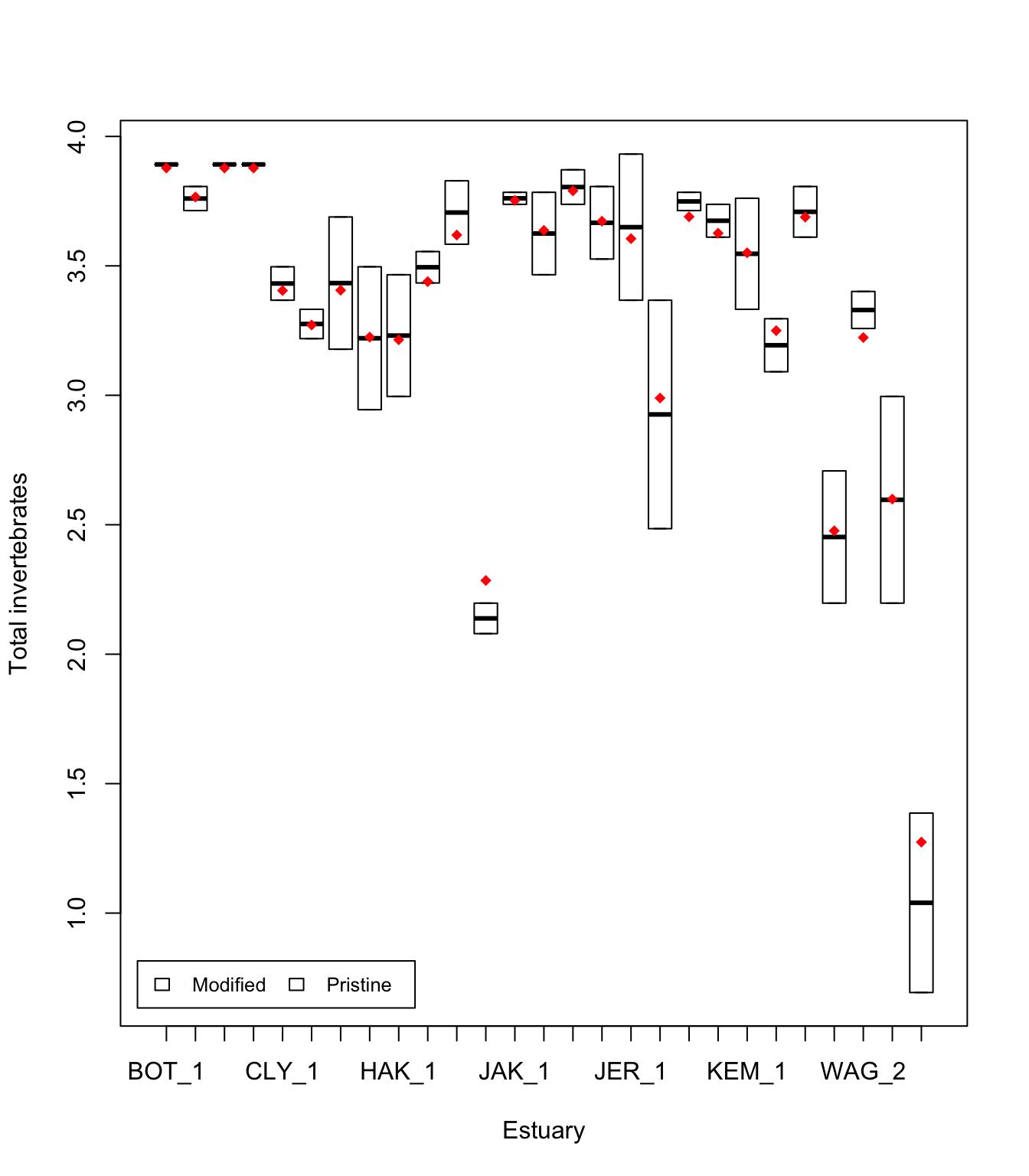
Alternatively, you can plot by Estuary as before (see Mixed models 1).
Further help
You can type ?lmer into R for help with these functions.
Draft book chapter from the authors of lme4.
Faraway, JJ (2005) Extending the linear model with R: generalized linear, mixed effects and nonparametric regression models. CRC Press.
Zuur, A, EN Ieno and GM Smith (2007) Analysing ecological data. Springer Science & Business Media.
Author: Gordana Popovic
Year: 2016
Last updated: Feb 2022