Generalised Mixed Models
Generalised linear mixed models
You will need to read Mixed models 1 and Mixed models 2 as an introduction to mixed models for continuous data, as well as the help pages on Generalised linear models as an introduction to modelling discrete data.
This page will combine the two to allow you to model discrete data (e.g., presence/absence) with random effects using generalised linear mixed models (GLMMs).
Properties of mixed models
Assumptions. The assumptions of generalised linear mixed models are a combination of the assumptions of GLMs and mixed models.
- The observed \(y\) are independent, conditional on some predictors \(x\)
- The response \(y\) come from a known distribution from the exponential family, with a known mean variance relationship
- There is a straight line relationship between some known function (link) of the mean of \(y\) and the predictors \(x\) and random effects \(z\)
- Random effects \(z\) are independent of \(y\).
- Random effects \(z\) are normally distributed
###Running the analysis
We will analyse the same data set as the first two mixed model tutorials. This data set aimed to test the effect of water pollution on the abundance of some subtidal marine invertebrates by comparing samples from modified and pristine estuaries. In the first two tutorials, we analysed the total count of invertebrates, which we assumed to be continuous as the total counts were large. Here, we will analyse the counts and presence/absences of individual species, which require generalised linear mixed models.
We will use the package lme4 for all our mixed effect modelling. It allows us to model both continuous and discrete data with one or more random effects. There are however some limitations for discrete data.
What lme4 can do
* model binary data (e.g., presence/absence)
* model counts with Poisson distribution
What lme4 can’t do
* model overdispersed counts (unfortunately these are really common in ecology)
* provide good residual plots (we need these for assumption checking)
First, load the package:
library(lme4)Download the sample data set, Estuaries.csv, and load into R.
Estuaries <- read.csv("Estuaries.csv", header = T)In this example, we have a fixed effect (Modification; modified vs pristine) and a random effect (Estuary). To test whether there is an effect of modification on individual species counts and presence/absences, we need to use generalised linear mixed models with the with the glmer function.

Consider the counts of hydroids (the variable Hydroid).
##  [1] 0 0 0 0 1 1 0 0 7 5 2 0 0 0 3 3 0 0 0 0 0 0 0 0 0 0 1 1 2 1 2 2 0 0 0 0 0 0
## [39] 0 0 0 0 1 0 0 0 0 3 1 0 1 2 2 2
Looking at the data, you can see the counts are small, with many zeros, so we don’t want to treat these as continuous. We will model them as counts with a Poisson distribution, and also as presence/absence data.
To model presence/absence, we first create a variable HydroidPres which is 1 (TRUE) when Hydroids are present and 0 (FALSE) otherwise.
Estuaries$HydroidPres <- Estuaries$Hydroid > 0Binary data
To fit a model for the presence or absence of hydroids, we would use glmer with family=binomial.
fit.bin <- glmer(HydroidPres ~ Modification + (1 | Estuary), family = binomial, data = Estuaries)Checking assumptions As usual, we can examine residual plots to check assumptions.
par(mfrow = c(1, 2))
plot(residuals(fit.bin) ~ fitted(fit.bin), main = "residuals v.s. Fitted")
qqnorm(residuals(fit.bin))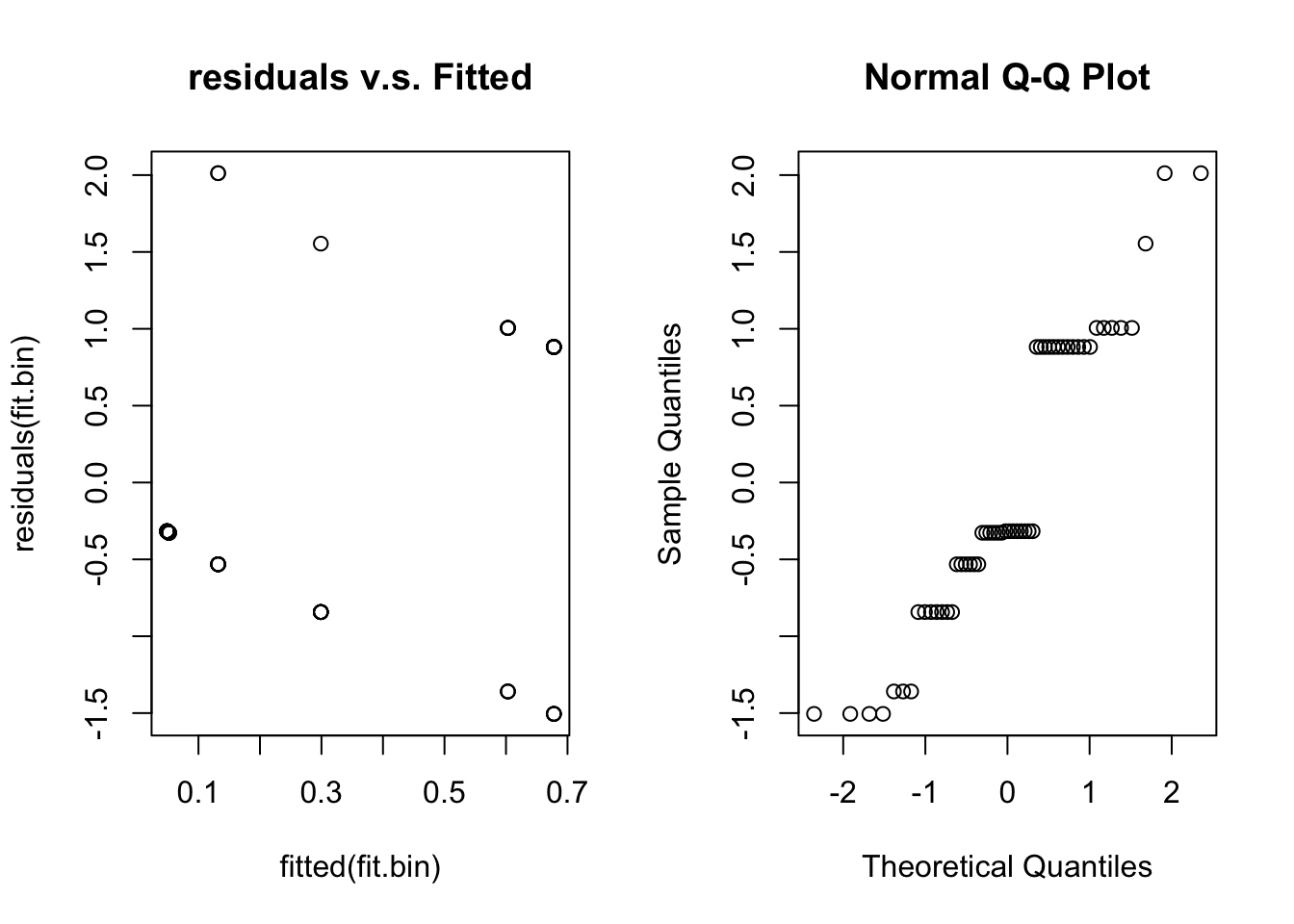
Unfortunately, for binary data residual plots are quite difficult to interpret. In the residual v.s. fitted plot all the 0’s are in a line (lower left) and all the ones are in a line (upper right) due to the discreteness of the data. This stops us from being able to look for patterns. We have the same problem with the normal quantile plot.
Briefly looking at our assumptions, Assumptions 1 and 4 we can’t check, but will be true if we sample randomly. Assumption 2 and 3 we should check with the residual plots, but given its failings we are unsure. Assumption 5 is hard to check in general and not crucial.
Hypothesis test for fixed effects
For generalised linear mixed models (GLMMs), we need to use the parametric bootstrap even for fixed effects inference. This is because the p-values from the anova function are quite approximate for GLMMs even for fixed effects. Sometimes the glmer function will give warnings or errors, so I’ve added a tryCatch to this code to handle that.
nBoot <- 1000
lrStat <- rep(NA, nBoot)
ft.null <- glmer(HydroidPres ~ 1 + (1 | Estuary), family = binomial, data = Estuaries) # null model
ft.alt <- glmer(HydroidPres ~ Modification + (1 | Estuary), family = binomial, data = Estuaries) # alternate model

lrObs <- 2 * logLik(ft.alt) - 2 * logLik(ft.null) # observed test stat

for (iBoot in 1:nBoot)
{
  Estuaries$HydroidPresSim <- unlist(simulate(ft.null)) # resampled data
  tryCatch(
    { # sometimes the glmer code doesn't converge

      bNull <- glmer(HydroidPresSim ~ 1 + (1 | Estuary), family = binomial, data = Estuaries) # null model
      bAlt <- glmer(HydroidPresSim ~ Modification + (1 | Estuary), family = binomial, data = Estuaries) # alternate model
      lrStat[iBoot] <- 2 * logLik(bAlt) - 2 * logLik(bNull) # resampled test stat
    },
    warning = function(war) {
      lrStat[iBoot] <- NA
    },
    error = function(err) {
      lrStat[iBoot] <- NA
    }
  ) # if code doesn't converge skip sim
}
mean(lrStat > lrObs, na.rm = T) # P-value for test of Estuary effect
## [1] 0.03089245We have evidence of an effect of modification on the presence of hydroids.
Count data
lme4 can model count data that has a Poisson distribution. If the data do not fit the Poisson mean/variance relationship, then things become much more complicated, and we won’t cover that situation here.
To model the counts of hydroids, we would use use glmer with family=poisson.
fit.pois <- glmer(Hydroid ~ Modification + (1 | Estuary), family = poisson, data = Estuaries)To check the assumptions:
par(mfrow = c(1, 2))
plot(residuals(fit.pois) ~ fitted(fit.pois), main = "Residuals vs. Fitted")
qqnorm(residuals(fit.pois))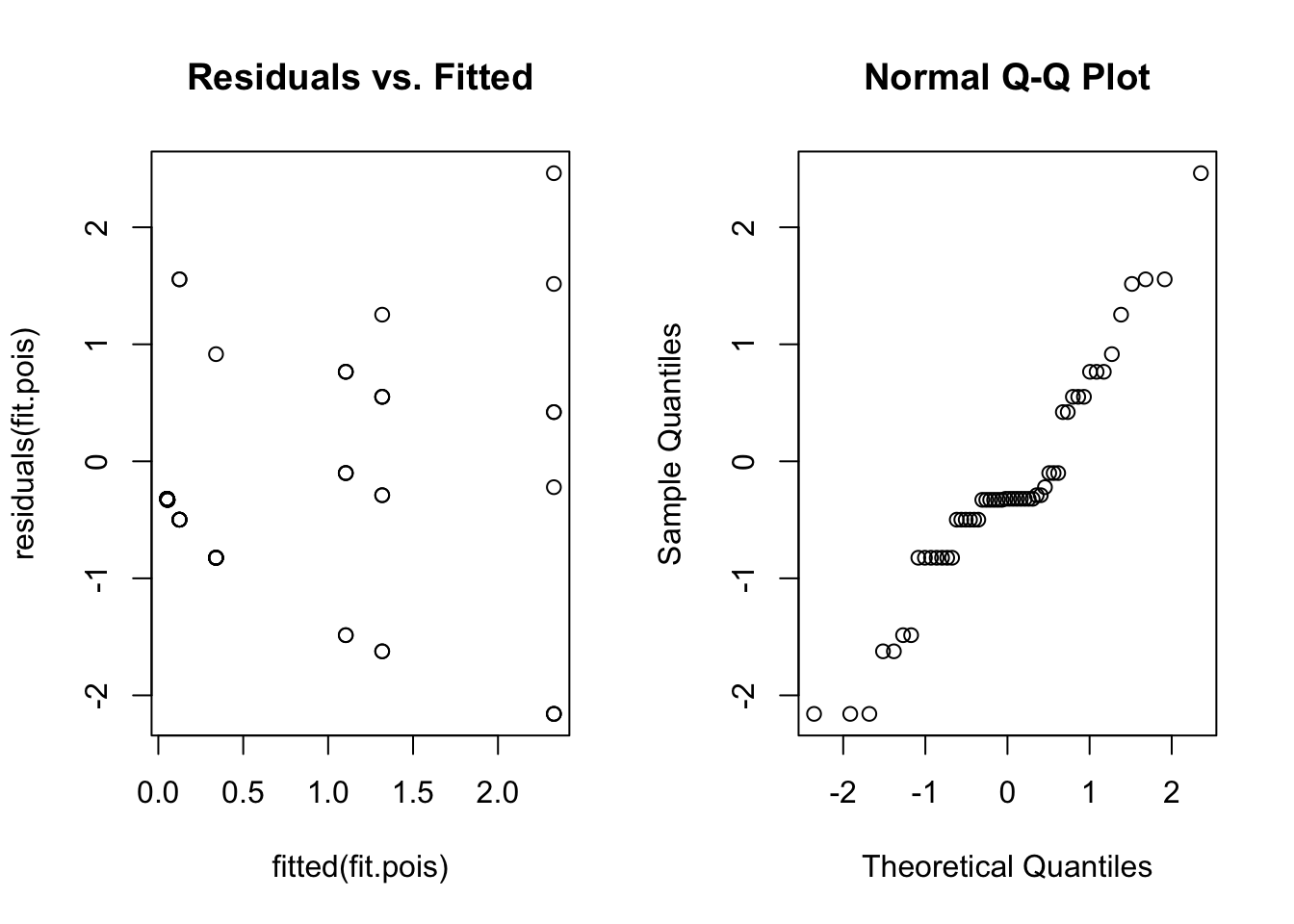
Once again, the residual plots aren’t that useful, but we at least get an idea about whether the variance assumption is reasonable. There is no obvious fan shape, so a Poisson model seems okay.
Hypothesis test for fixed effects
Again, we can use parametric bootstrapping to test for an effect of Modification.
nBoot <- 1000
lrStat <- rep(NA, nBoot)
ft.null <- glmer(Hydroid ~ 1 + (1 | Estuary), family = poisson, data = Estuaries) # null model
ft.alt <- glmer(Hydroid ~ Modification + (1 | Estuary), family = poisson, data = Estuaries) # alternate model

lrObs <- 2 * logLik(ft.alt) - 2 * logLik(ft.null) # observed test stat
for (iBoot in 1:nBoot)
{
  Estuaries$HydroidSim <- unlist(simulate(ft.null)) # resampled data
  tryCatch(
    {
      bNull <- glmer(HydroidSim ~ 1 + (1 | Estuary), family = poisson, data = Estuaries) # null model
      bAlt <- glmer(HydroidSim ~ Modification + (1 | Estuary), family = poisson, data = Estuaries) # alternate model
      lrStat[iBoot] <- 2 * logLik(bAlt) - 2 * logLik(bNull) # resampled test stat
    },
    warning = function(war) {
      lrStat[iBoot] <- NA
    },
    error = function(err) {
      lrStat[iBoot] <- NA
    }
  ) # if code doesn't converge skip sim#   lrStat[iBoot]
}
## boundary (singular) fit: see ?isSingular
## boundary (singular) fit: see ?isSingular
## boundary (singular) fit: see ?isSingular
## boundary (singular) fit: see ?isSingular
## boundary (singular) fit: see ?isSingular
## boundary (singular) fit: see ?isSingular
## boundary (singular) fit: see ?isSingular
## boundary (singular) fit: see ?isSingular
## boundary (singular) fit: see ?isSingular
## boundary (singular) fit: see ?isSingular
## boundary (singular) fit: see ?isSingular
## boundary (singular) fit: see ?isSingular
## boundary (singular) fit: see ?isSingular
## boundary (singular) fit: see ?isSingular
## boundary (singular) fit: see ?isSingular
## boundary (singular) fit: see ?isSingular
## boundary (singular) fit: see ?isSingular
## boundary (singular) fit: see ?isSingular
## boundary (singular) fit: see ?isSingular
## boundary (singular) fit: see ?isSingular
## boundary (singular) fit: see ?isSingular
## boundary (singular) fit: see ?isSingular
## boundary (singular) fit: see ?isSingular
## boundary (singular) fit: see ?isSingular
## boundary (singular) fit: see ?isSingular
## boundary (singular) fit: see ?isSingular
## boundary (singular) fit: see ?isSingular
## boundary (singular) fit: see ?isSingular
## boundary (singular) fit: see ?isSingular
## boundary (singular) fit: see ?isSingular
## boundary (singular) fit: see ?isSingular
## boundary (singular) fit: see ?isSingular
## boundary (singular) fit: see ?isSingular
## boundary (singular) fit: see ?isSingular
## boundary (singular) fit: see ?isSingular
## boundary (singular) fit: see ?isSingular
## boundary (singular) fit: see ?isSingular
## boundary (singular) fit: see ?isSingular
## boundary (singular) fit: see ?isSingular
## boundary (singular) fit: see ?isSingular
## boundary (singular) fit: see ?isSingular
## boundary (singular) fit: see ?isSingular
## boundary (singular) fit: see ?isSingular
## boundary (singular) fit: see ?isSingular
## boundary (singular) fit: see ?isSingular
## boundary (singular) fit: see ?isSingular
## boundary (singular) fit: see ?isSingular
## boundary (singular) fit: see ?isSingular
## boundary (singular) fit: see ?isSingular
## boundary (singular) fit: see ?isSingular
## boundary (singular) fit: see ?isSingular
## boundary (singular) fit: see ?isSingular
## boundary (singular) fit: see ?isSingular
## boundary (singular) fit: see ?isSingular
## boundary (singular) fit: see ?isSingular
## boundary (singular) fit: see ?isSingular
## boundary (singular) fit: see ?isSingular
## boundary (singular) fit: see ?isSingular
## boundary (singular) fit: see ?isSingular
## boundary (singular) fit: see ?isSingular
## boundary (singular) fit: see ?isSingular
## boundary (singular) fit: see ?isSingular
## boundary (singular) fit: see ?isSingular
## boundary (singular) fit: see ?isSingular
## boundary (singular) fit: see ?isSingular
## boundary (singular) fit: see ?isSingular
## boundary (singular) fit: see ?isSingular
## boundary (singular) fit: see ?isSingular
## boundary (singular) fit: see ?isSingular
## boundary (singular) fit: see ?isSingular
## boundary (singular) fit: see ?isSingular
## boundary (singular) fit: see ?isSingular
## boundary (singular) fit: see ?isSingular
## boundary (singular) fit: see ?isSingular
## boundary (singular) fit: see ?isSingular
## boundary (singular) fit: see ?isSingular
## boundary (singular) fit: see ?isSingular
## boundary (singular) fit: see ?isSingular
## boundary (singular) fit: see ?isSingular
## boundary (singular) fit: see ?isSingular
## boundary (singular) fit: see ?isSingular
## boundary (singular) fit: see ?isSingularmean(lrStat > lrObs, na.rm = TRUE) # P-value for test of Estuary effect## [1] 0.04202719We have evidence of an effect of modification on hydroid abundance.
A non Poisson example
Often, count data will not fit a Poisson distribution. Look at what happens if you try and model the counts of the bryozoan, Schizoporella errata, from that same data set.
fit.pois2 <- glmer(Schizoporella.errata ~ Modification + (1 | Estuary), family = poisson, data = Estuaries)
par(mfrow = c(1, 2))
plot(residuals(fit.pois) ~ fitted(fit.pois), main = "residuals vs. Fitted")
qqnorm(residuals(fit.pois))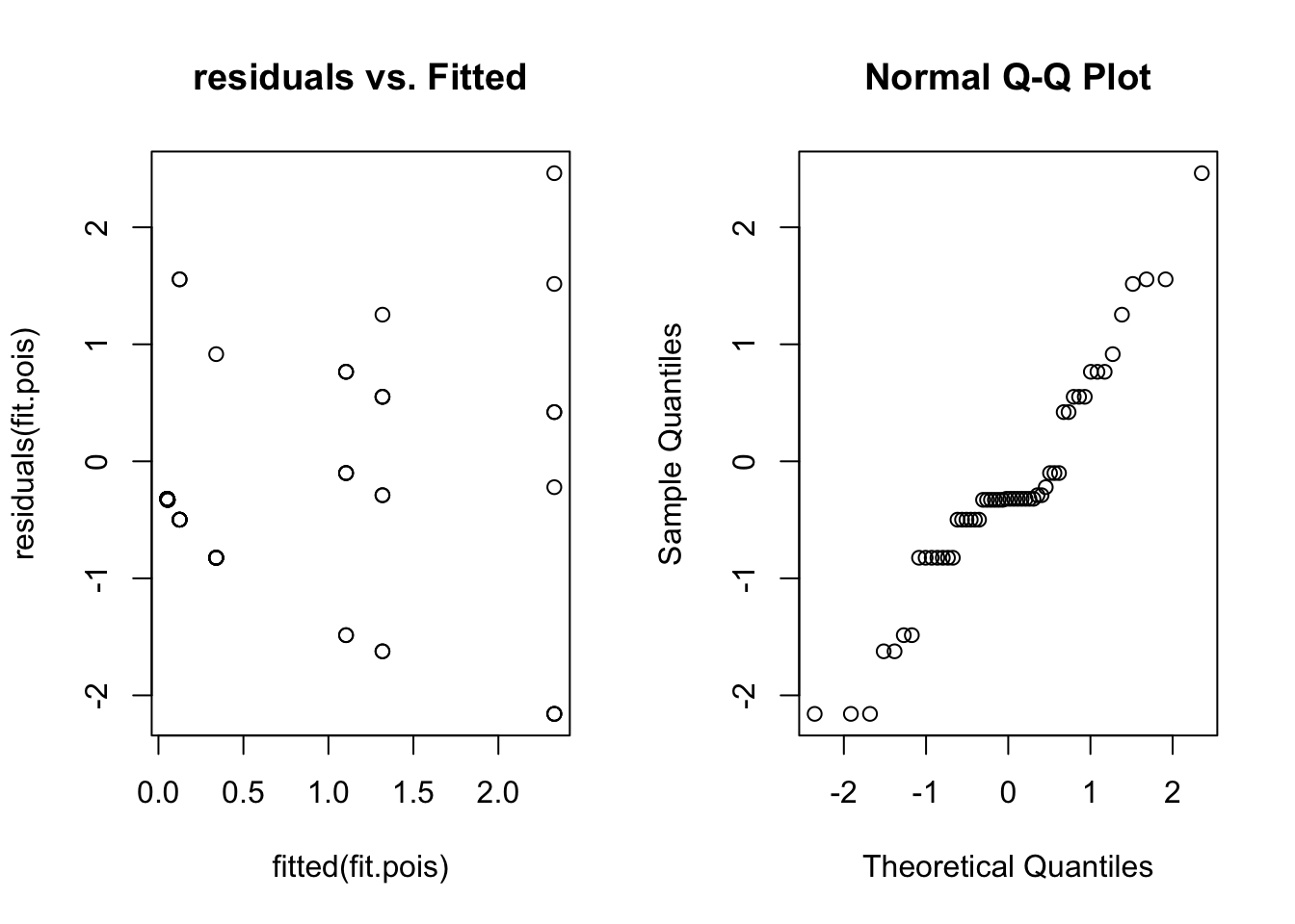
Here we can see a distinct fan shape in the residual vs. fitted plot. Unfortunately lme4 can’t handle this situation (overdispersion), and there is no easy way to model these data. If this happens in your data try the glmmADMB package.
Hypothesis test for random effects
As before you could run hypothesis tests on the random effects using a parametric bootstrap. See Mixed models 1 and Mixed models 2 for code that you could modify for this situation.
###Communicating results
Written. Results of generalised linear mixed models are communicated in a similar way to results for linear models. In your results section you should mention that you are using mixed models with R package lme4, and list your random and fixed effects. You should also mention how you carried out inference, i.e. likelihood ratio tests (using the anova) or parametric bootstrap. In the results section for one predictor, it suffices to write one line, e.g. “There is strong evidence (p<0.001) of negative effect of modification on total abundance”. For multiple predictors it’s best to display the results in a table.
Visual. The best way to visually communicate results will depend on your question, for a simple mixed model with one random effect, a plot of the raw data with the model means superimposed is one possibility.
library(Hmisc)
fit.pois <- glmer(Hydroid ~ Modification + (1 | Estuary), family = poisson, data = Estuaries)
means <- fitted(fit.pois) # this will give the estimate at each data point
ModEst <- unique(Estuaries[c("Estuary", "Modification")]) # find which Estuaries are modified
cols <- as.numeric(ModEst[order(ModEst[, 1]), 2]) + 3 # Assign colour by modification
## Warning: NAs introduced by coercionboxplot(Hydroid ~ Estuary, data = Estuaries, col = cols, xlab = "Estuary", ylab = "Count of hydroids")
legend("topleft",
inset = .02,
c("Modified", "Pristine"), fill = unique(cols), horiz = TRUE, cex = 0.8
)
Est.means <- summarize(means, Estuaries$Estuary, mean)$means # extract means by Estuary
stripchart(Est.means ~ sort(unique(Estuary)), data = Estuaries, pch = 18, col = "red", vertical = TRUE, add = TRUE) # plot means by estuary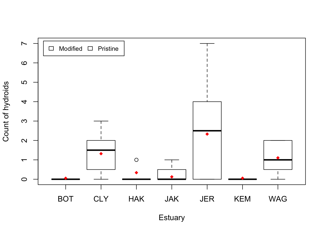
Further help
You can type ?glmer into R for help with this function.
Draft book chapter from the authors of lme4.
Faraway, JJ (2005) Extending the linear model with R: generalized linear, mixed effects and nonparametric regression models. CRC Press.
Zuur, A, EN Ieno and GM Smith (2007) Analysing ecological data. Springer Science & Business Media.
Author: Gordana Popovic
Year: 2016
Last updated: Feb 2022