Paired T-test
Paired t-tests are used to compare the means of two groups of measurements when individual objects are measured twice, once for each type of measurement. Data could be paired in various ways: if the same measure is taken from a single object in two different treatments or at two different times, or if different types of measures are being contrasted from the same object.

For example, to contrast the photosynthetic performance of ten plants in two environments in a greenhouse (shady and sunny), we could measure performance in each individual plant twice, once in the shade and once in the sun. The measures are paired by belonging to the same individual plant.
For this experimental design, we would use a paired t-test to compare the measurements taken in the two environments. The 20 individual measurements are not independent of each other because we would expect the pair of measurements taken from the same individual to be more similar to each other than if randomly sampled from all available plants. We are thus unable to use an independent samples t test - that test would be appropriate if each plant was used only once, with some plants measured in the shady treatment and different set of plants measured in the sunny treatment.
Pairing data like this is usually done to reduce the likely variation among measurements with the aim of better detecting differences between groups. In this example, the difference between the two measures of photosynthetic performance on a given plant should reflect mostly the effect of sunlight, while in an independent samples design, the difference between a plant in the shade and another plant in the sun will reflect both differences in the effects of sunlight and differences between the individual plants.
For a paired t-test, the test statistic, t is:
\[t = \frac{\bar{d}}{SE_{d}}\]
Where the \(\bar{d}\) is the mean of the differences between values for each pair, and SEd is the standard error of that set of differences.
Note that this equation is identical to a One sample t-test, used to contrast any sample mean (\(\bar{x}\)) to a known population mean (\(\mu\)) or hypothesised value. What you are doing here is testing whether your sample of differences is likely to have come from a population of differences that have a mean of zero (another way of saying that your groups are the same).
\[t = \frac{\bar{x}-\mu}{SE}\]
Running the analysis
The test statistic t is relatively straightforward to calculate manually. The test statistic can then checked against a t distribution in order to determine the probability of obtaining that value of the test statistic if the null hypothesis is true. In R, to calculate the probability associated with a given value of t use:
pt(q, df = your.df, lower.tail = FALSE) * 2where q is your value of t, your.df is the degrees of freedom (the number of pairs-1). The lower.tail = FALSE ensures that you are calculating the probability of getting a t value larger than yours (i.e the upper tail, P[X > x]). Note that the critical value for t (\(\alpha = 0.05\)) varies depending on the number of degrees of freedom - larger degrees of freedom = smaller critical value of t.
The t.test function gives you the test statistic and its associated probability in one output. For an paired t-test, we would use:
t.test(x = my_sample1, y = my_sample2, paired = TRUE)where my_sample1 and my_sample2 are vectors containing the measurements from each sample. You would need to make sure the two vectors have the same number of values and that data from each pair were in the matching rows.
Alternatively, if you have a data frame with the response and predictor variables in separate columns you can use a formula statement, y ~ x, rather than the code above. Again, you would need to ensure the matching pairs were in the right order (e.g., the fourth row of the shady treatment is the data collected from the same plant as the fourth row of the sunny treatment).
Download a sample data set in this format, Greenhouse.csv, and import into R
Greenhouse <- read.csv(file = "Greenhouse.csv", header = TRUE)The paired t-test is run with the t.test function, with the arguments specifying the response variable (Performance) to the left of the ~, the predictor variable (Treatment) to the right of the ~, the data frame to be used and the fact that it is a paired t-test.
t.test(Performance ~ Treatment, data = Greenhouse, paired = TRUE)Interpreting the results
##
##  Paired t-test
##
## data:  Performance by Treatment
## t = -18.812, df = 9, p-value = 1.557e-08
## alternative hypothesis: true difference in means is not equal to 0
## 95 percent confidence interval:
##  -0.2111674 -0.1658326
## sample estimates:
## mean of the differences
##                 -0.1885
The important output of a paired t-test includes the test statistic t, in this case 18.8, the degrees of freedom (in this case 9) and the probability associated with that value of t. In this case, we have a very low p value (p < 0.001) and can reject the null hypothesis that the plants can photosynthesise with the same performance in the two light environments.
You also get the mean and 95% confidence intervals for the differences between measurements in each pair (this will not overlap zero when the test is significant).
Assumptions to check
t-tests are parametric tests, which implies we can specify a probability distribution for the population of the variable from which samples were taken. Parametric (and non-parametric) tests have a number of assumptions. If these assumptions are violated we can no longer be sure that the test statistic follows a t distribution, in which case p-values may be inaccurate.
Normality. For a paired t-test, it is assumed the the sample of differences is normally distributed. If these are highly skewed, transformations may be used to achieve a distribution closer to normal.
Independence. The paired design takes into account that the two measures from each pair are not independent. It is still important, however, that each pair of objects measured are independent from other pairs. If they are linked in any way (e.g., groups of plants sharing a water tray) then more complex analytical design that account for additional factors may be required.
Communicating the results
Written. As a minimum, the observed t statistic, the P-value and the number of degrees of freedom should be reported. For example, you could write “The photosynthetic performance of plants was significantly greater in sunny environments in contrast to shady environments (paired t-test: t = 18.81, df = 9, P < 0.001)”.
Visual. Box plots or column graphs with error bars are effective ways of communicating the variation in a single continuous response variable versus a single categorical predictor variable.
boxplot(Performance ~ Treatment, data = Greenhouse, xlab = "Light environment", ylab = "Photosynthetic performance (FvFm)")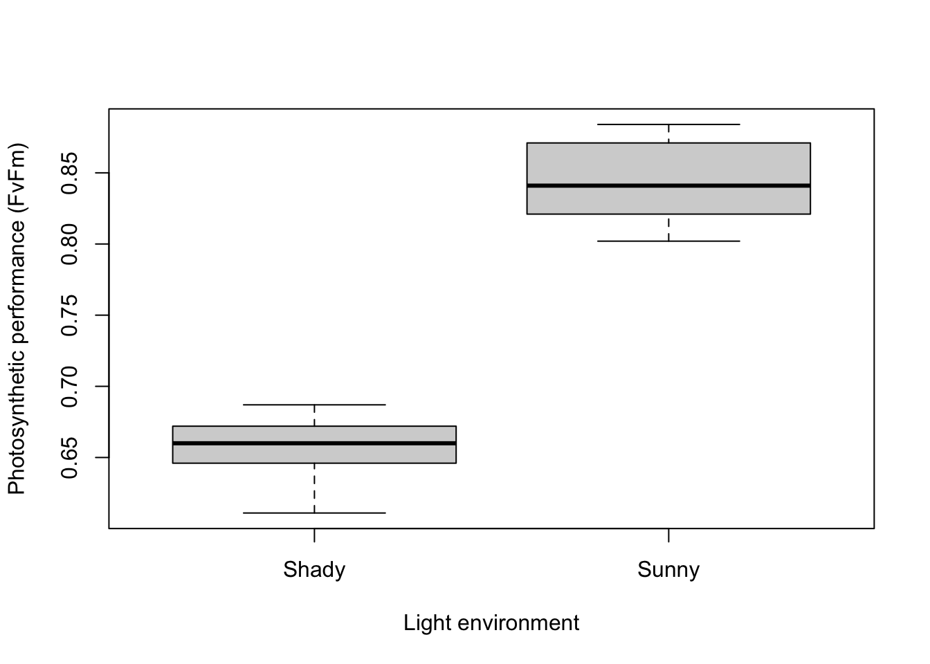
Further help
Type ?t.test to get the R help for this function.
Quinn and Keough (2002) Experimental design and data analysis for biologists. Cambridge University Press. Chapter 9: Hypothesis testing.
McKillup (2012) Statistics explained. An introductory guide for life scientists. Cambridge University Press. Chapter 9: Comparing the means of one and two samples of normally distributed data.
Author: Alistair Poore
Year: 2016
Last updated: Feb 2022