Interpreting Linear Regressions
The interpretation of coefficients in (generalized) linear models is more subtle than you many realise, and has consequences for how we test hypotheses and report findings. We will start by talking about marginal vs. conditional interpretations of model parameters.

In this example, we model plant height as a function of altitude and temperature. These variables are negatively correlated: it is colder the higher you go. We start by simulating some data to reflect this.
library(mvtnorm)

# Specify the sample size
N <- 1000

# Specify the correlation between altitude and temperature
rho <- -0.4

# This line of code creates two correlated variables
X <- rmvnorm(N, mean = c(0, 0), sigma = matrix(c(1, rho, rho, 1), 2, 2))

# Extract the first and second columns to vectors named temp and alt and plot
temp <- X[, 1]
alt <- X[, 2]
plot(temp, alt)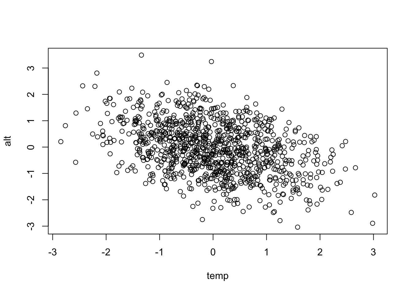
Now we can simulate some data for height of plants. Here we say that the mean height of plants is 2 (when all the other variables are 0), as temperature increases by one unit (holding altitude constant), the mean of height will increase by 1 unit (beta[2] = 1), and similarly as you increase altitude by 1 unit (holding temperature constant) then mean height decreases by 1 (beta[3] = -1). Height is then normally distributed with this mean and standard deviation of 2.
beta <- c(2, 1, -1)
mu <- beta[1] + beta[2] * temp + beta[3] * alt
height <- rnorm(N, mu, sd = 2)
If we use a linear model to find the coefficients we get what we expect, estimates very close to the true values.
lm_both <- lm(height ~ temp + alt)
data.frame(estimated = round(lm_both$coefficients, 2), true = beta)
## estimated true
## (Intercept) 1.93 2
## temp 1.05 1
## alt -1.00 -1The interpretation of these coefficients is that if you hold everything else in the model constant (i.e., temperature) and add 1 to altitude, then the estimated mean height will decrease by 1.09. Note that the coefficient depends on the units in which altitude is measured. If altitude is in meters then the coefficient tells you what happens when you go up 1 meter.
The intercept is the predicted value when all the other variables are set to 0, which sometimes makes sense (here it would be the height of plants at sea level and 0 temperature). Other times 0 is not a meaningful value, and if you would like to interpret the intercept it might make sense to rescale your other variables so that their mean is 0. If you do this, then the intercept is the predicted value when all other variables are at their mean level.
What if now we had a model with just temperature?
lm1 <- lm(height ~ temp)
lm1$coefficients
## (Intercept) temp
## 1.976334 1.458025The coefficient of temperature is now 1.38, what’s going on? Altitude is an important predictor of plant height, and some of the information about altitude is contained in temperature (remember they are correlated, so as altitude increases temperature decreases). The model accounts for this by changing the effect of temperature to take account of the information it contains about altitude. Notice the coefficient of temperature is wrong by approximately 0.4, the amount of correlation between the variables.
Note: When statisticians talk about this, they use the words conditional and marginal. Conditional is the effect of a variable when others are held constant (as in lm_both), while marginal is the overall effect (as in lm1). Note: If you use the code above to simulate your own data sets, you will get slightly different values for the coefficients.
Testing hypotheses
This distinction has a lot of consequences for modelling as well as testing hypothesis. Let’s generate some data where altitude predicts height, and temperature has no (additional) information, and then test for temperature.
mu <- 2 - 1 * alt
height <- rnorm(N, mu, sd = 2)

mod_temp <- lm(height ~ temp)
summary(mod_temp)
##
## Call:
## lm(formula = height ~ temp)
##
## Residuals:
## Min 1Q Median 3Q Max
## -6.7462 -1.6037 -0.0034 1.5473 6.8263
##
## Coefficients:
## Estimate Std. Error t value Pr(>|t|)
## (Intercept) 2.07071 0.07078 29.256 < 2e-16 ***
## temp 0.48267 0.07348 6.569 8.13e-11 ***
## ---
## Signif. codes: 0 '***' 0.001 '**' 0.01 '*' 0.05 '.' 0.1 ' ' 1
##
## Residual standard error: 2.238 on 998 degrees of freedom
## Multiple R-squared: 0.04145, Adjusted R-squared: 0.04049
## F-statistic: 43.15 on 1 and 998 DF, p-value: 8.134e-11anova(mod_temp)## Analysis of Variance Table
##
## Response: height
## Df Sum Sq Mean Sq F value Pr(>F)
## temp 1 216.2 216.19 43.153 8.134e-11 ***
## Residuals 998 4999.7 5.01
## ---
## Signif. codes: 0 '***' 0.001 '**' 0.01 '*' 0.05 '.' 0.1 ' ' 1The output of this model is telling us there is an effect of temperature, even though technically there isn’t. It is not giving us false information if you understand how to interpret model outputs. Because temperature is correlated with altitude, and there is an effect of altitude, when altitude is not in the model, the model tells us overall there is an effect of temperature of increasing height by 0.45 (remember the correlation was 0.4). If our hypothesis is ‘Does plant height change with temperature?’, the answer is yes, the higher the temperature, the taller the plants.
But what about altitude? We know the temperature effect we observe is because it is correlated with altitude, temperature does not directly predict height. If we want to know if there is an effect of temperature after controlling for altitude (holding altitude constant, so conditional), then we fit the model with altitude and then test for temperature.
mod_temp_alt <- lm(height ~ alt + temp)
summary(mod_temp_alt)
##
## Call:
## lm(formula = height ~ alt + temp)
##
## Residuals:
## Min 1Q Median 3Q Max
## -6.1044 -1.4496 0.0178 1.3228 6.7075
##
## Coefficients:
## Estimate Std. Error t value Pr(>|t|)
## (Intercept) 2.02439 0.06379 31.736 <2e-16 ***
## alt -1.06246 0.06938 -15.313 <2e-16 ***
## temp 0.05128 0.07190 0.713 0.476
## ---
## Signif. codes: 0 '***' 0.001 '**' 0.01 '*' 0.05 '.' 0.1 ' ' 1
##
## Residual standard error: 2.015 on 997 degrees of freedom
## Multiple R-squared: 0.224, Adjusted R-squared: 0.2224
## F-statistic: 143.9 on 2 and 997 DF, p-value: < 2.2e-16anova(mod_temp_alt)## Analysis of Variance Table
##
## Response: height
## Df Sum Sq Mean Sq F value Pr(>F)
## alt 1 1166.1 1166.08 287.2182 <2e-16 ***
## temp 1 2.1 2.07 0.5087 0.4759
## Residuals 997 4047.7 4.06
## ---
## Signif. codes: 0 '***' 0.001 '**' 0.01 '*' 0.05 '.' 0.1 ' ' 1The p-value is about 0.95, so we have no evidence of an effect of temperature after controlling for altitude.
Note: The distinction between conditional and marginal interpretations is also true for generalised linear models and mixed models.
Categorical covariates
When we have categorical covariates (for example treatment), there are a number of ways to code the model, which will give different interpretations for the coefficients. Let’s simulate 120 data points with 40 in each of three levels of a categorical treatment.
N <- 120
# The effect of treatment
trt.n <- rep(c(-1, 0, 1), N / 3)
mu <- 2 + 1 * trt.n

# Labels for the treatment
treatment <- factor(rep(c("low", "med", "high"), N / 3)) # group labels

# Create, Y, a normally distributed response variable and plot against treatment
Y <- rnorm(N, mu, sd = 2)
boxplot(Y ~ treatment)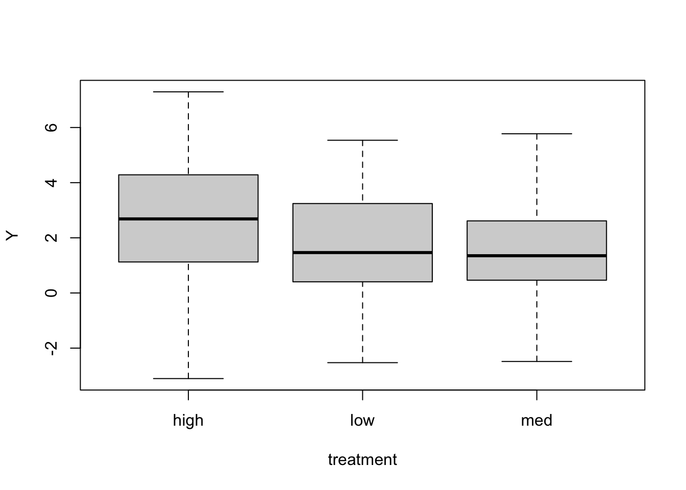
If we put treatment in as a covariate the normal way, the model will choose a reference treatment (here it will be high as the levels get sorted alphabetically), so that the intercept will be the mean of this reference group. The other coefficients will be the differences between the other groups and the reference group.
cat_lm <- lm(Y ~ treatment)
summary(cat_lm)
##
## Call:
## lm(formula = Y ~ treatment)
##
## Residuals:
## Min 1Q Median 3Q Max
## -5.6953 -1.2191 -0.1793 1.2402 4.7025
##
## Coefficients:
## Estimate Std. Error t value Pr(>|t|)
## (Intercept) 2.5913 0.3189 8.126 5.18e-13 ***
## treatmentlow -0.9398 0.4510 -2.084 0.0393 *
## treatmentmed -1.0175 0.4510 -2.256 0.0259 *
## ---
## Signif. codes: 0 '***' 0.001 '**' 0.01 '*' 0.05 '.' 0.1 ' ' 1
##
## Residual standard error: 2.017 on 117 degrees of freedom
## Multiple R-squared: 0.05116, Adjusted R-squared: 0.03494
## F-statistic: 3.154 on 2 and 117 DF, p-value: 0.04633So here group “high” has a mean of 2.65, and the difference between the means of group “low” and group “high” is -0.66, and the difference between group “med” and group “high” is -1.48. If you would like to have another group as the reference group, you can use relevel to recode your treatment factor.
treatment <- relevel(treatment, ref = "low")
cat_lm <- lm(Y ~ treatment)
summary(cat_lm)
##
## Call:
## lm(formula = Y ~ treatment)
##
## Residuals:
## Min 1Q Median 3Q Max
## -5.6953 -1.2191 -0.1793 1.2402 4.7025
##
## Coefficients:
## Estimate Std. Error t value Pr(>|t|)
## (Intercept) 1.65144 0.31890 5.179 9.42e-07 ***
## treatmenthigh 0.93981 0.45099 2.084 0.0393 *
## treatmentmed -0.07769 0.45099 -0.172 0.8635
## ---
## Signif. codes: 0 '***' 0.001 '**' 0.01 '*' 0.05 '.' 0.1 ' ' 1
##
## Residual standard error: 2.017 on 117 degrees of freedom
## Multiple R-squared: 0.05116, Adjusted R-squared: 0.03494
## F-statistic: 3.154 on 2 and 117 DF, p-value: 0.04633boxplot(Y ~ treatment)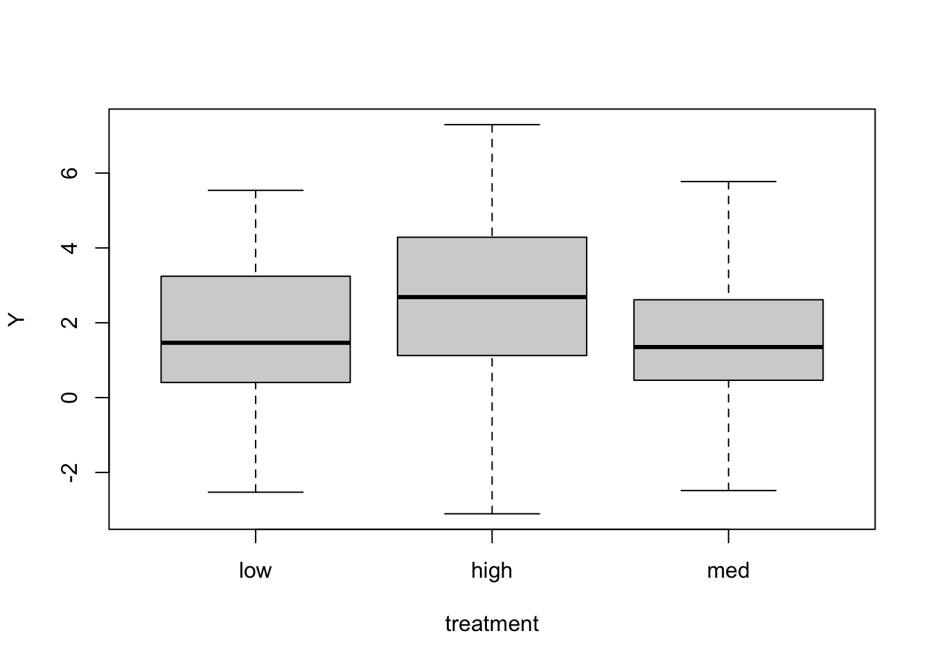
Now the intercept is the mean of group “low”, and all the other coefficients are the differences between group “low” and the others. Another thing you can do is to put -1 in the model to get rid of the intercept, and just have the means of each group as coefficients.
cat_lm <- lm(Y ~ treatment - 1)
summary(cat_lm)
##
## Call:
## lm(formula = Y ~ treatment - 1)
##
## Residuals:
## Min 1Q Median 3Q Max
## -5.6953 -1.2191 -0.1793 1.2402 4.7025
##
## Coefficients:
## Estimate Std. Error t value Pr(>|t|)
## treatmentlow 1.6514 0.3189 5.179 9.42e-07 ***
## treatmenthigh 2.5913 0.3189 8.126 5.18e-13 ***
## treatmentmed 1.5737 0.3189 4.935 2.68e-06 ***
## ---
## Signif. codes: 0 '***' 0.001 '**' 0.01 '*' 0.05 '.' 0.1 ' ' 1
##
## Residual standard error: 2.017 on 117 degrees of freedom
## Multiple R-squared: 0.5004, Adjusted R-squared: 0.4876
## F-statistic: 39.07 on 3 and 117 DF, p-value: < 2.2e-16Now, the three coefficients are the mean of the groups.
Contrasting the coefficients We can also look at contrasts; these are the difference between all pairs of groups. Load the package multcomp and use glht (general linear hypotheses) to examine all pair-wise differences.
library(multcomp)

cont <- glht(cat_lm, linfct = mcp(treatment = "Tukey"))

summary(cont)
##
## Simultaneous Tests for General Linear Hypotheses
##
## Multiple Comparisons of Means: Tukey Contrasts
##
##
## Fit: lm(formula = Y ~ treatment - 1)
##
## Linear Hypotheses:
## Estimate Std. Error t value Pr(>|t|)
## high - low == 0 0.93981 0.45099 2.084 0.0976 .
## med - low == 0 -0.07769 0.45099 -0.172 0.9838
## med - high == 0 -1.01750 0.45099 -2.256 0.0662 .
## ---
## Signif. codes: 0 '***' 0.001 '**' 0.01 '*' 0.05 '.' 0.1 ' ' 1
## (Adjusted p values reported -- single-step method)Each line of this output compares two groups against one another. The first line, for example, compares the “high” group to the “low” group. So the difference between the means of the “high” and “low” groups is 1.84. The p-values and the confidence intervals given byglht control for multiple testing, which is handy. If you want to see the confidence intervals for the differences between the groups.
confint(cont)##
## Simultaneous Confidence Intervals
##
## Multiple Comparisons of Means: Tukey Contrasts
##
##
## Fit: lm(formula = Y ~ treatment - 1)
##
## Quantile = 2.3739
## 95% family-wise confidence level
##
##
## Linear Hypotheses:
## Estimate lwr upr
## high - low == 0 0.93981 -0.13081 2.01043
## med - low == 0 -0.07769 -1.14831 0.99293
## med - high == 0 -1.01750 -2.08812 0.05312Note: In a model with multiple covariates, the same rules still apply in terms of conditional and marginal interpretations of coefficients.
Interpreting coefficients in generalised linear models In linear models, the interpretation of model parameters is linear, as discussed above. For generalised linear models, now read the tutorial page on interpreting coefficients in those models.
Author: Gordana Popovic
Year: 2016
Last updated: Feb 2022