Generalised Additive Models (GAMs)
Many data in the environmental sciences do not fit simple linear models and are best described by “wiggly models”, also known as Generalised Additive Models (GAMs).
Let’s start with a famous tweet by one Gavin Simpson, which amounts to:
1. GAMs are just GLMs
2. GAMs fit wiggly terms
3. use + s(x) not x in your syntax
4. use method = "REML"
5. always look at gam.check()
This is basically all there is too it - an extension of generalised linear models (GLMs) with a smoothing function. Of course, there may be many sophisticated things going on when you fit a model with smooth terms, but you only need to understand the rationale and some basic theory. There are also lots of what would be apparently magic things happening when we try to understand what is under the hood of say lmer or glmer, but we use them all the time without reservation!
GAMs in a nutshell
Let’s start with an equation for a Gaussian linear model: \[y = \beta_0 + x_1\beta_1 + \varepsilon, \quad \varepsilon \sim N(0, \sigma^2)\] What changes in a GAM is the presence of a smoothing term: \[y = \beta_0 + f(x_1) + \varepsilon, \quad \varepsilon \sim N(0, \sigma^2)\] This simply means that the contribution to the linear predictor is now some function \(f\). This is not that dissimilar conceptually to using a quadratic (\(x_1^2\)) or cubic term (\(x_1^3\)) as your predictor.
The function \(f\) can be something more funky or kinky - here, we’re going to focus on splines. In the old days, it might have been something like piecewise linear functions.
You can have combinations of linear and smooth terms in your model, for example \[y = \beta_0 + x_1\beta_1 + f(x_2) + \varepsilon, \quad \varepsilon \sim N(0, \sigma^2)\] or we can fit generalised distributions and random effects, for example \[ln(y) = \beta_0 + f(x_1) + \varepsilon, \quad \varepsilon \sim Poisson(\lambda)\] \[ln(y) = \beta_0 + f(x_1) + z_1\gamma + \varepsilon, \quad \varepsilon \sim Poisson(\lambda), \quad \gamma \sim N(0,\Sigma)\]
A simple example
Lets try a simple example. First, let’s create a data frame and fill it with some simulated data with an obvious non-linear trend and compare how well some models fit to that data.
x <- seq(0, pi * 2, 0.1)
sin_x <- sin(x)
y <- sin_x + rnorm(n = length(x), mean = 0, sd = sd(sin_x / 2))
Sample_data <- data.frame(y, x)
library(ggplot2)
ggplot(Sample_data, aes(x, y)) +
geom_point()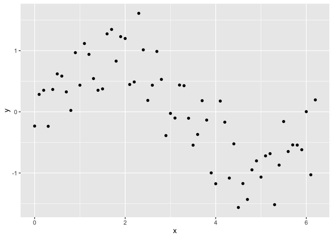
Try fitting a normal linear model:
lm_y <- lm(y ~ x, data = Sample_data)and plotting the fitted line with data using geom_smooth in ggplot
ggplot(Sample_data, aes(x, y)) +
  geom_point() +
  geom_smooth(method = lm)
## `geom_smooth()` using formula 'y ~ x'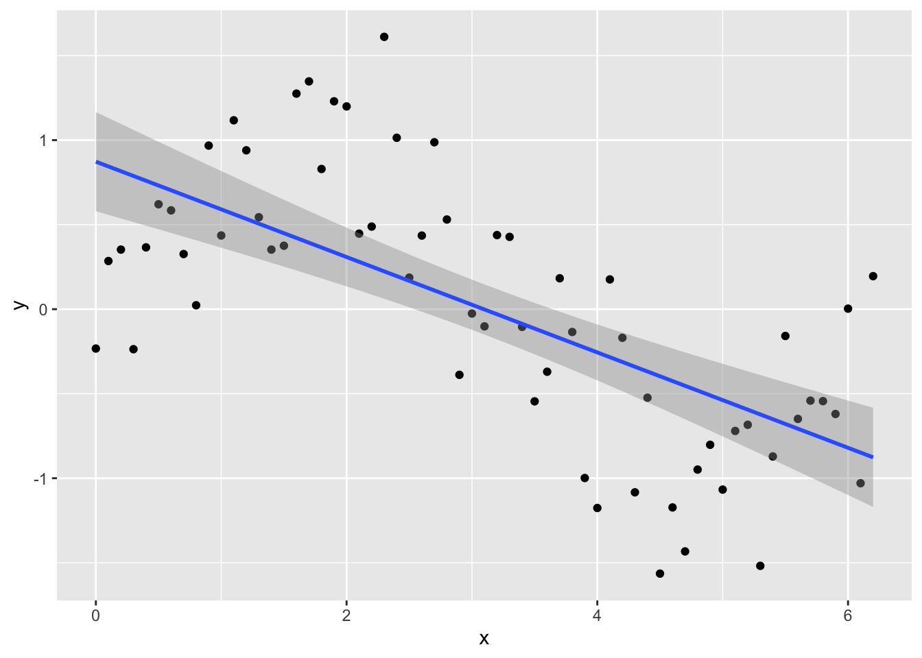
Looking at the plot or summary(lm_y), you might think the model fits nicely, but look at the residual plot - eek!
plot(lm_y, which = 1)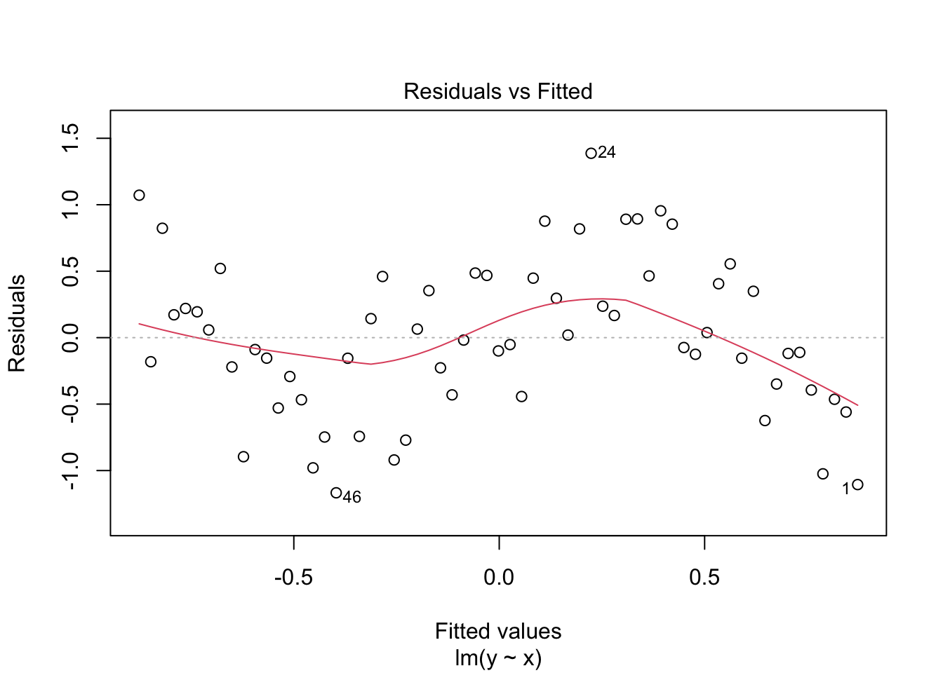
Clearly, the residuals are not evenly spread across values of \(x\), and we need to consider a better model.
Running the analysis
Before we consider a GAM, we need to load the package mgcv - the choice for running GAMs in R.
library(mgcv)To run a GAM, we use:
gam_y <- gam(y ~ s(x), method = "REML")To extract the fitted values, we can use predict just like normal:
x_new <- seq(0, max(x), length.out = 100)
y_pred <- predict(gam_y, data.frame(x = x_new))
But for simple models, we can also utilise the method = argument in geom_smooth, specifying the model formula.
ggplot(Sample_data, aes(x, y)) +
  geom_point() +
  geom_smooth(method = "gam", formula = y ~ s(x))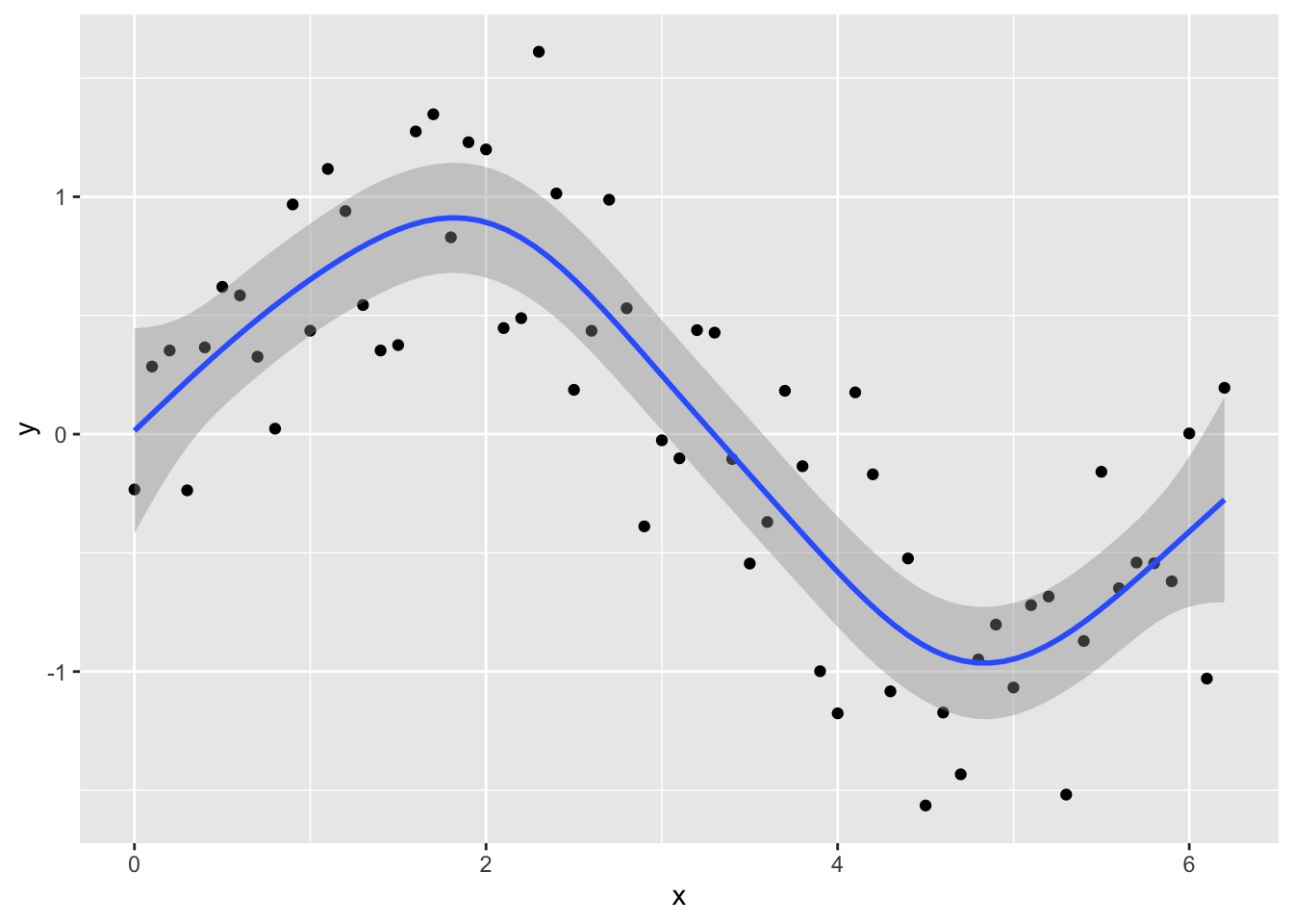
You can see the model is better fit to the data, but always check the diagnostics.
check.gam is quick and easy to view the residual plots.
par(mfrow = c(2, 2))
gam.check(gam_y)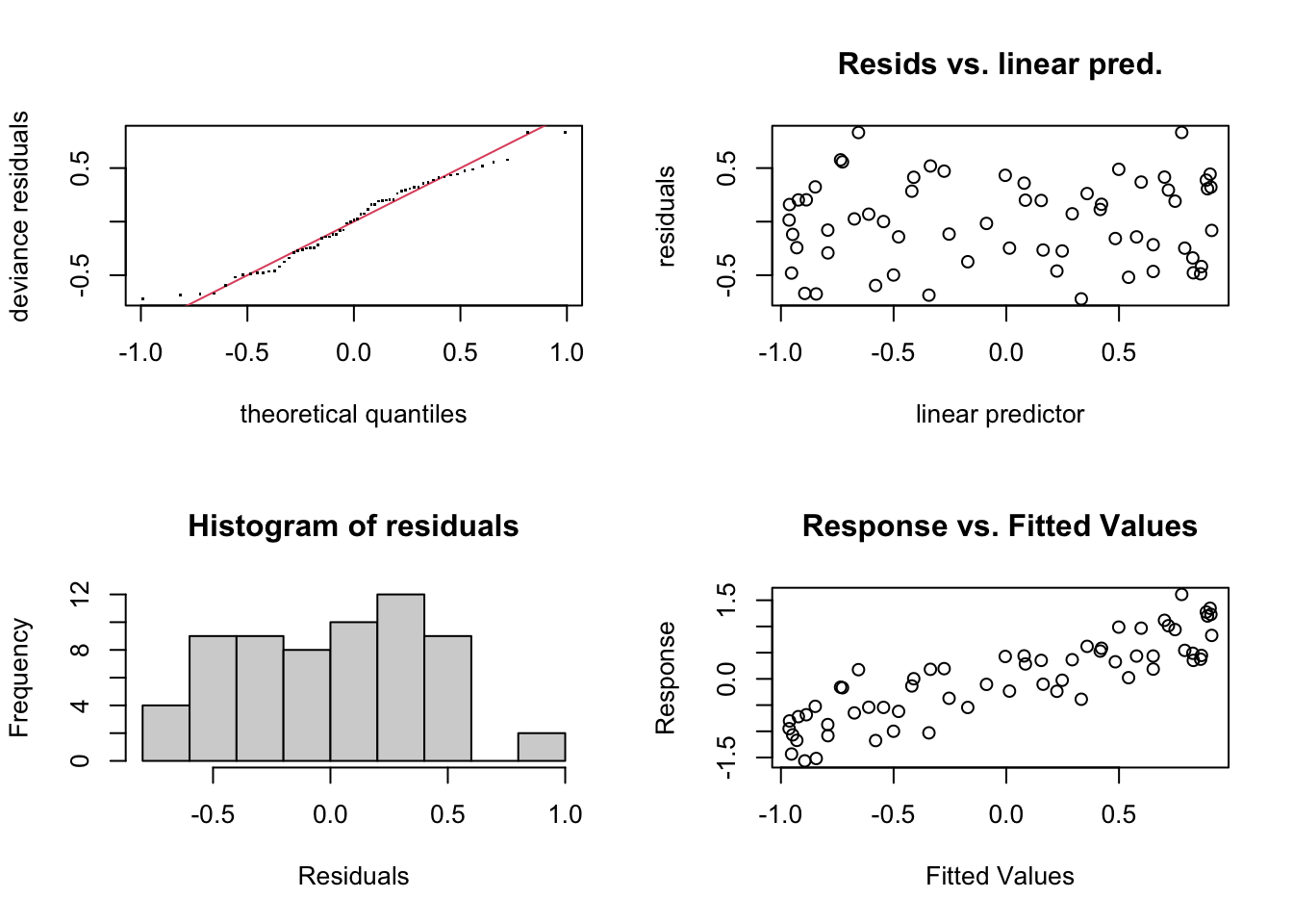
##
## Method: REML   Optimizer: outer newton
## full convergence after 6 iterations.
## Gradient range [-1.414605e-09,8.821477e-11]
## (score 42.06195 & scale 0.1691468).
## Hessian positive definite, eigenvalue range [1.940833,30.65633].
## Model rank =  10 / 10
##
## Basis dimension (k) checking results. Low p-value (k-index<1) may
## indicate that k is too low, especially if edf is close to k'.
##
##        k'  edf k-index p-value
## s(x) 9.00 5.23    1.06    0.65
Using summary with the model object will give you the significance of the smooth term (along with any parametric terms, if you’ve included them), along with the variance explained. In this example, a pretty decent fit. The ‘edf’ is the estimated degrees of freedom - essentially, the larger the number, the more wiggly the fitted model. Values of around 1 tend to be close to a linear term. You can read about penalisation and shrinkage for more on what the edf reflects.
summary(gam_y)##
## Family: gaussian
## Link function: identity
##
## Formula:
## y ~ s(x)
##
## Parametric coefficients:
## Estimate Std. Error t value Pr(>|t|)
## (Intercept) -0.001923 0.051816 -0.037 0.971
##
## Approximate significance of smooth terms:
## edf Ref.df F p-value
## s(x) 5.226 6.345 25.54 <2e-16 ***
## ---
## Signif. codes: 0 '***' 0.001 '**' 0.01 '*' 0.05 '.' 0.1 ' ' 1
##
## R-sq.(adj) = 0.722 Deviance explained = 74.6%
## -REML = 42.062 Scale est. = 0.16915 n = 63Smooth terms
As mentioned above, we’ll focus on splines, as they are the smooth functions that are most commonly implemented (and are pretty quick and stable). So what was actually going on when we specified s(x)?
Well, this is where we say we want to fit \(y\) as a linear function of some set of functions of \(x\). The default in mgcv is a thin plate regression spline - the two common ones you’ll probably see are these, and cubic regression splines. Cubic regression splines have the traditional knots that we think of when we talk about splines - they’re evenly spread across the covariate range in this case. We’ll just stick to thin plate regression splines, since I figure Simon made them the default for a reason,
Basis functions OK, so here’s where we see what the wiggle bit is really made of. We’ll start with the fitted model, then we’ll look at it from first principles (not really). Remembering that the smooth term is the sum of some number of functions (I’m not sure how well this equation really represents the smooth term, but you get the point), \[f(x_1) = \sum_{j=1}^kb_j(x_1)\beta_j\] First we extract the set of basis functions (that is, the \(b_j(x_j)\) part of the smooth term). Then we can plot say the first and second basis functions.
model_matrix <- predict(gam_y, type = "lpmatrix")
plot(y ~ x)
abline(h = 0)
lines(x, model_matrix[, "s(x).1"], type = "l", lty = 2)
lines(x, model_matrix[, "s(x).2"], type = "l", lty = 2)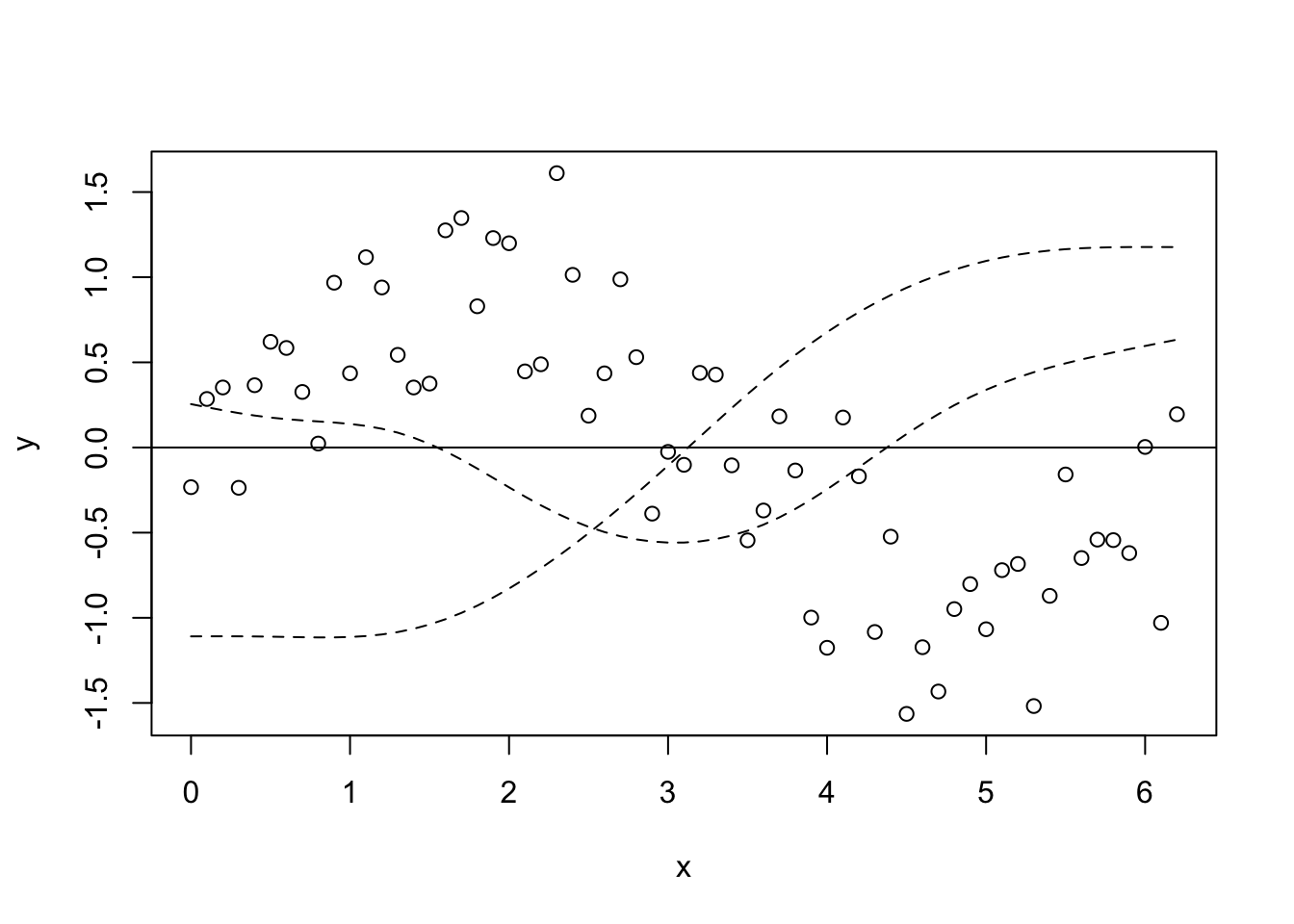
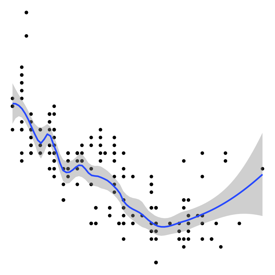
Let’s plot all of the basis functions now, and then add that to the predictions from the GAM (y_pred) on top again.
plot(y ~ x)
abline(h = 0)

x_new <- seq(0, max(x), length.out = 100)
y_pred <- predict(gam_y, data.frame(x = x_new))

matplot(x, model_matrix[, -1], type = "l", lty = 2, add = T)
lines(y_pred ~ x_new, col = "red", lwd = 2)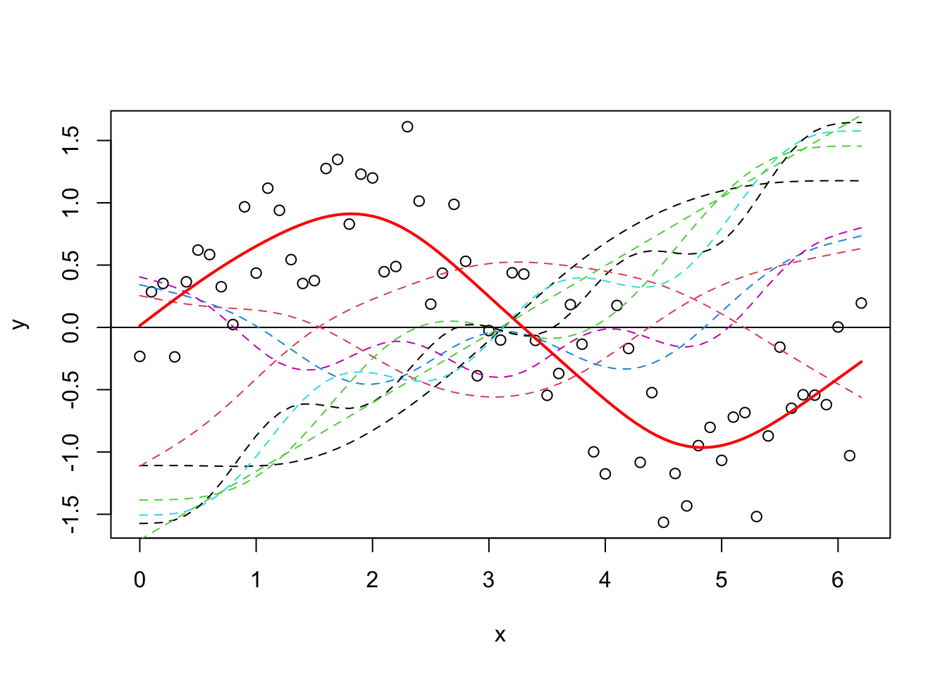
Now, it’s difficult at first to see what has happened, but it’s easiest to think about it like this - each of those dotted lines represents a function (\(b_j\)) for which gam estimates a coefficient (\(\beta_j\)), and when you sum them you get the contribution for the corresponding \(f(x)\) (i.e. the previous equation). It’s nice and simple for this example, because we model \(y\) only as a function of the smooth term, so it’s fairly relatable. As an aside, you can also just use plot.gam to plot the smooth terms.
plot(gam_y)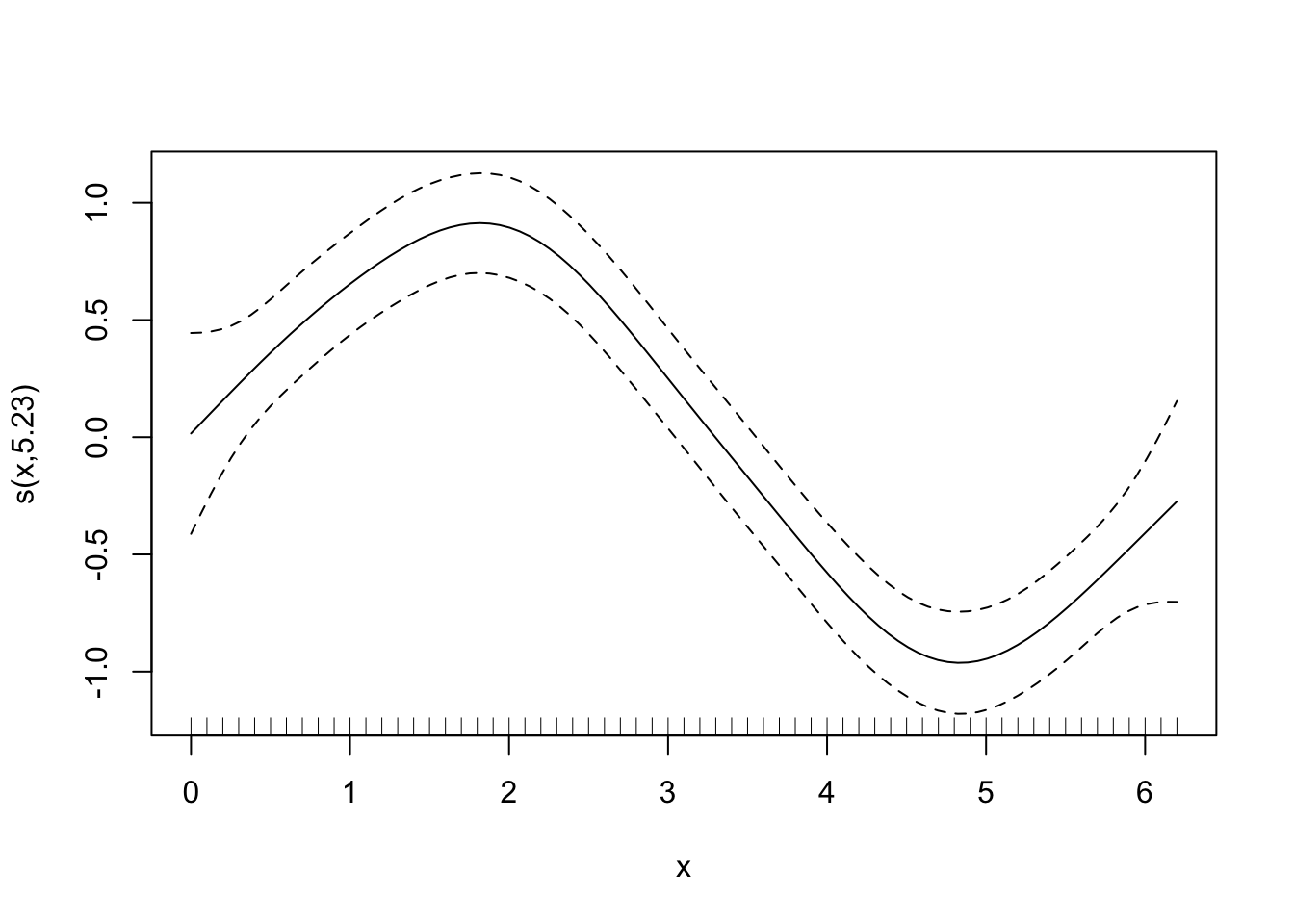
OK, now let’s look a little closer at how the basis functions are constructed. You’ll see that the construction of the functions is separate to the response data. Just to prove it, we’ll use smoothCon.
x_sin_smooth <- smoothCon(s(x), data = data.frame(x), absorb.cons = TRUE)
X <- x_sin_smooth[[1]]$X

par(mfrow = c(1, 2))
matplot(x, X, type = "l", main = "smoothCon()")
matplot(x, model_matrix[, -1], type = "l", main = "predict(gam_y)")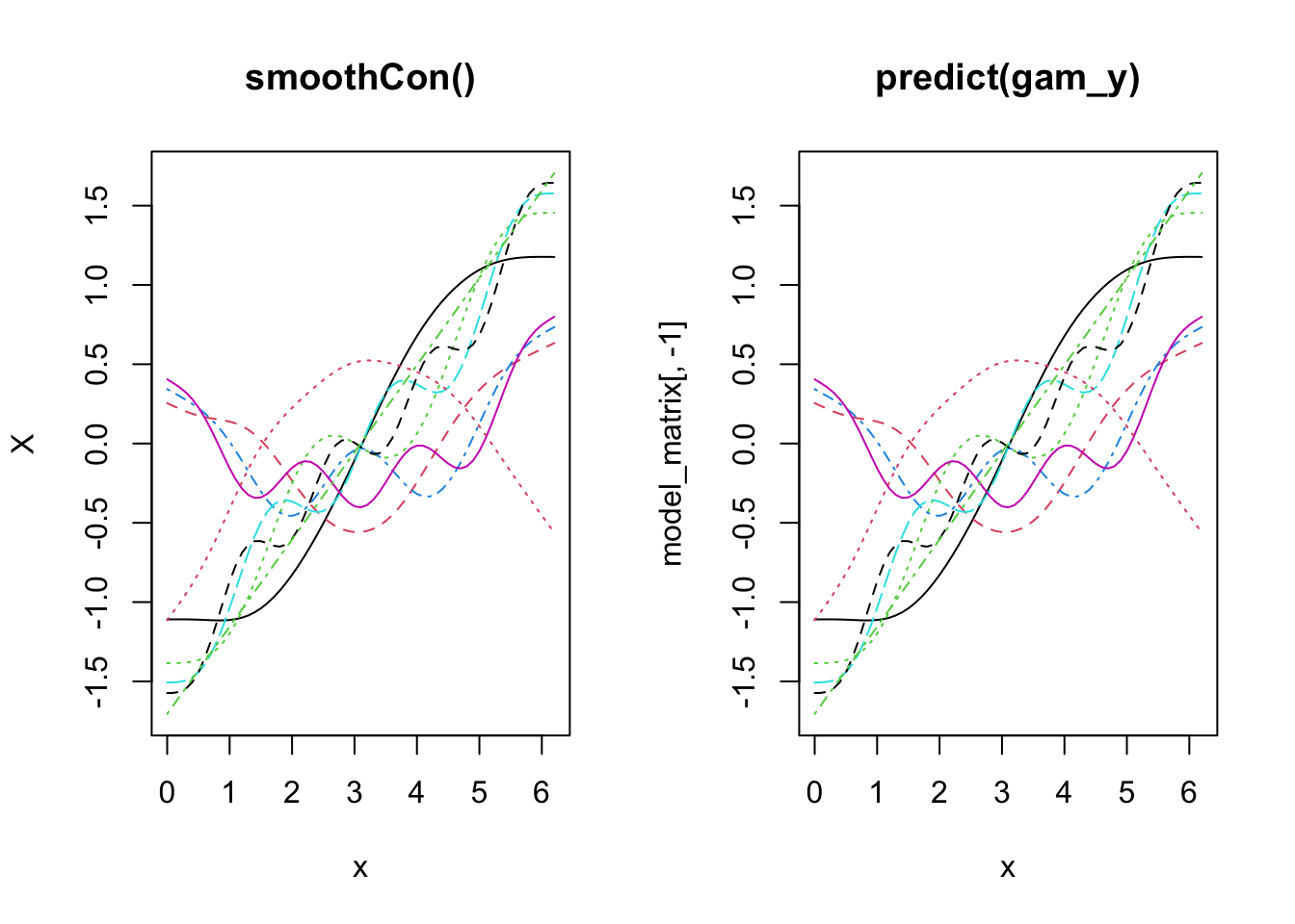
And now to prove that you can go from the basis functions and the estimated coefficients to the fitted smooth term. Again note that this is simplified here because the model is just one smooth term. If you had more terms, we would need to add up all of the terms in the linear predictor.
betas <- gam_y$coefficients
linear_pred <- model_matrix %*% betas

par(mfrow = c(1, 2))
plot(y ~ x, main = "manual from basis/coefs")
lines(linear_pred ~ x, col = "red", lwd = 2)
plot(y ~ x, main = "predict(gam_y)")
lines(y_pred ~ x_new, col = "red", lwd = 2)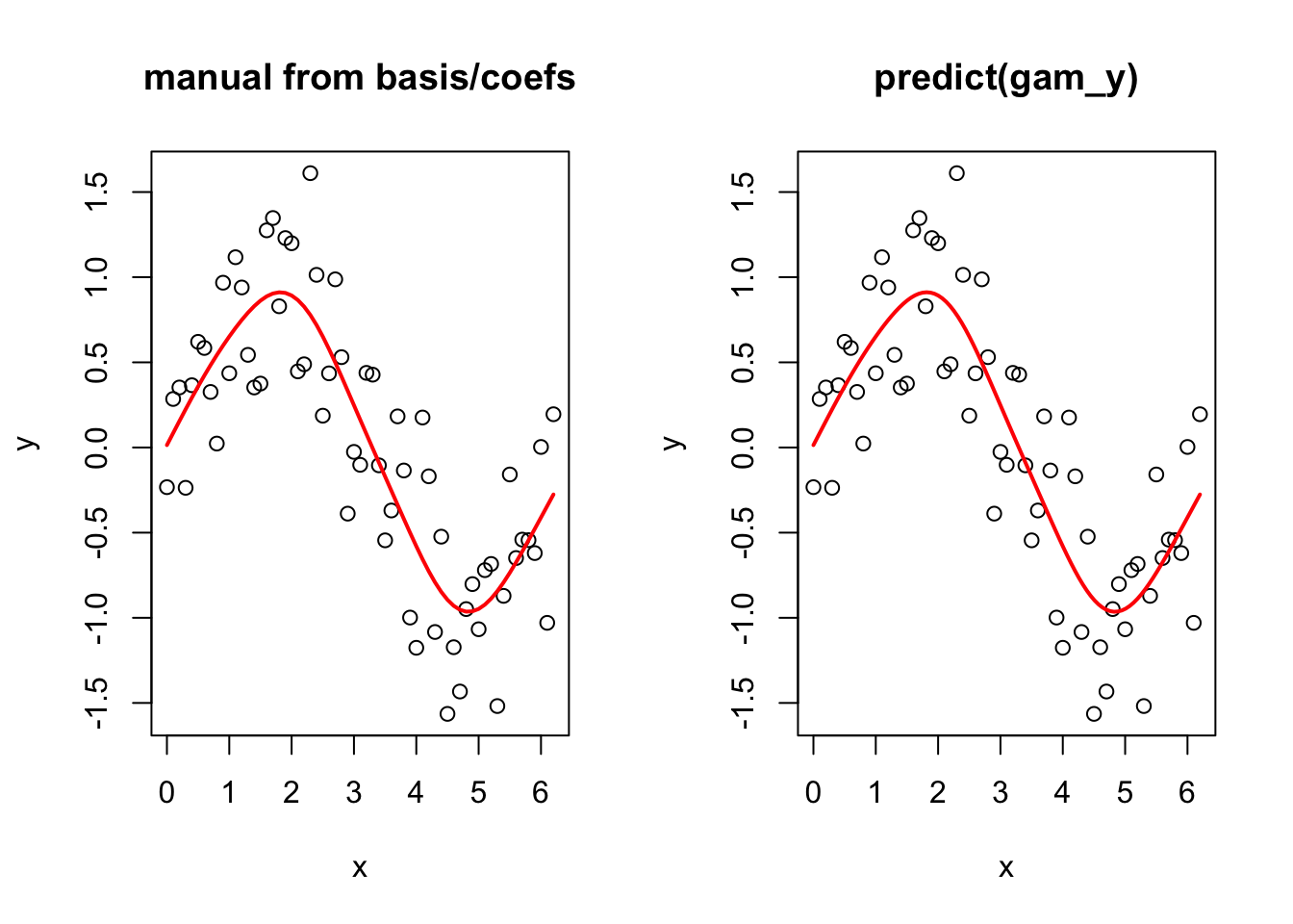
Out of interest, take a look at the following plot, remembering that X is the matrix of basis functions.
par(mfrow = c(1, 2))
plot(y ~ x)
plot(y ~ rowSums(X))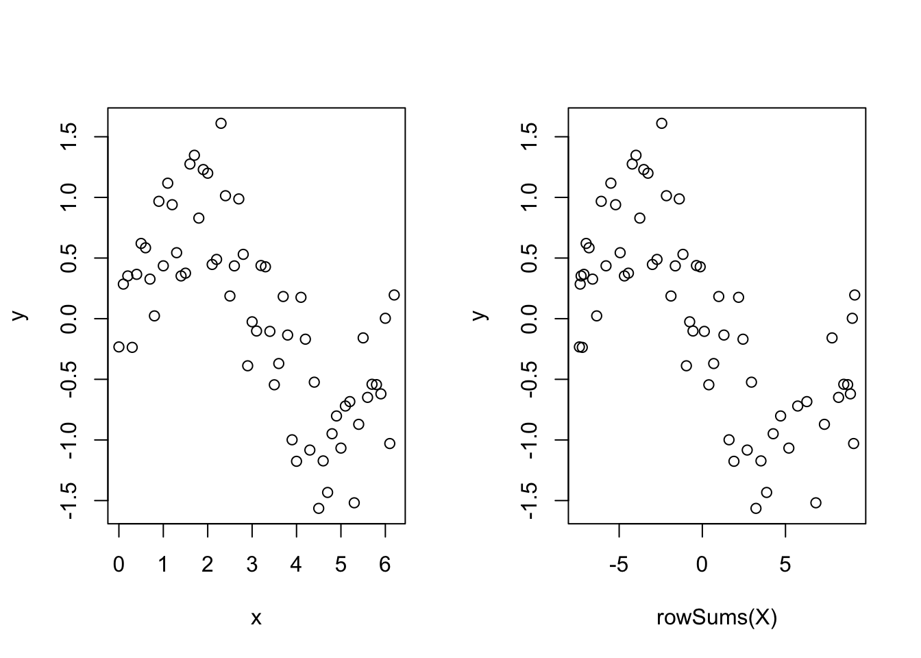
Not so scary huh? Of course this is not quite the whole story - see gam.models and smooth.terms to see all of the options for types of smoothers, how the basis functions are constructed (penalisation etc.), types of models we can specify (random effects, linear functionals, interactions, penalisation) plus much more.
A quick real example

We’ll now look at a quick real example - we’ll just scratch the surface, and in a future We’ll now look at a quick real example - we’ll just scratch the surface, and in a future tutorial we will look at it in more detail. We’re going to look at some CO\(_2\) data from Manua Loa. We will fit a couple GAMs to the data to try and pick apart the intra- and inter-annual trends.
First load the data - you can download it here.
CO2 <- read.csv("mauna_loa_co2.csv")We want to look at inter-annual trend first, so let’s convert the date into a continuous time variable (take a subset for visualisation).
CO2$time <- as.integer(as.Date(CO2$Date, format = "%d/%m/%Y"))
CO2_dat <- CO2
CO2 <- CO2[CO2$year %in% (2000:2010), ]
OK, so let’s plot it and look at a smooth term for time. \[y = \beta_0 + f_{\mathrm{trend}}(time) + \varepsilon, \quad \varepsilon \sim N(0, \sigma^2)\]
ggplot(CO2_dat, aes(time, co2)) +
  geom_line()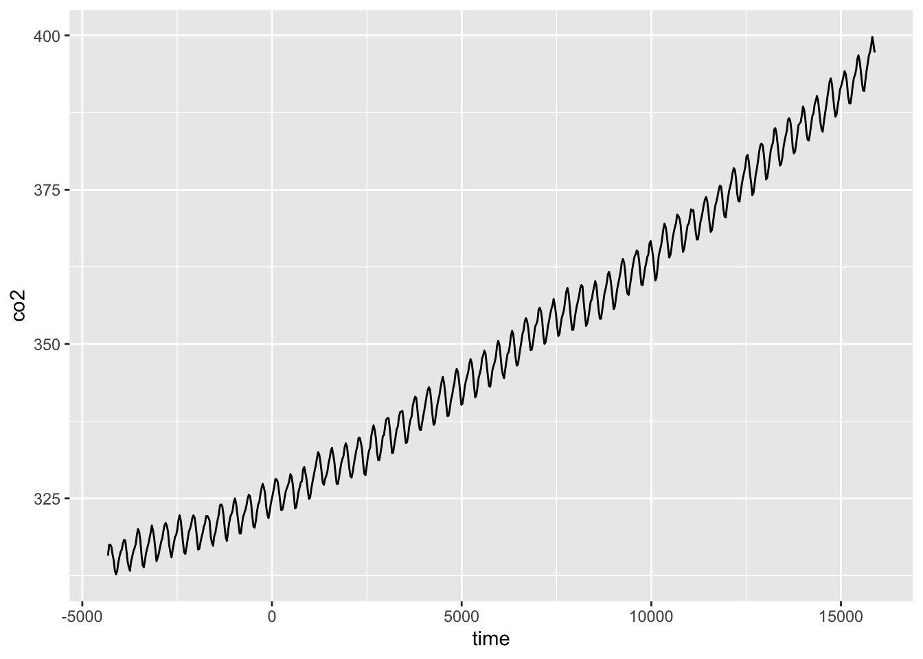
We can fit a GAM for these data using:
CO2_time <- gam(co2 ~ s(time), data = CO2, method = "REML")which fits a model with a single smooth term for time. We can look at the predicted values for this:
plot(CO2_time)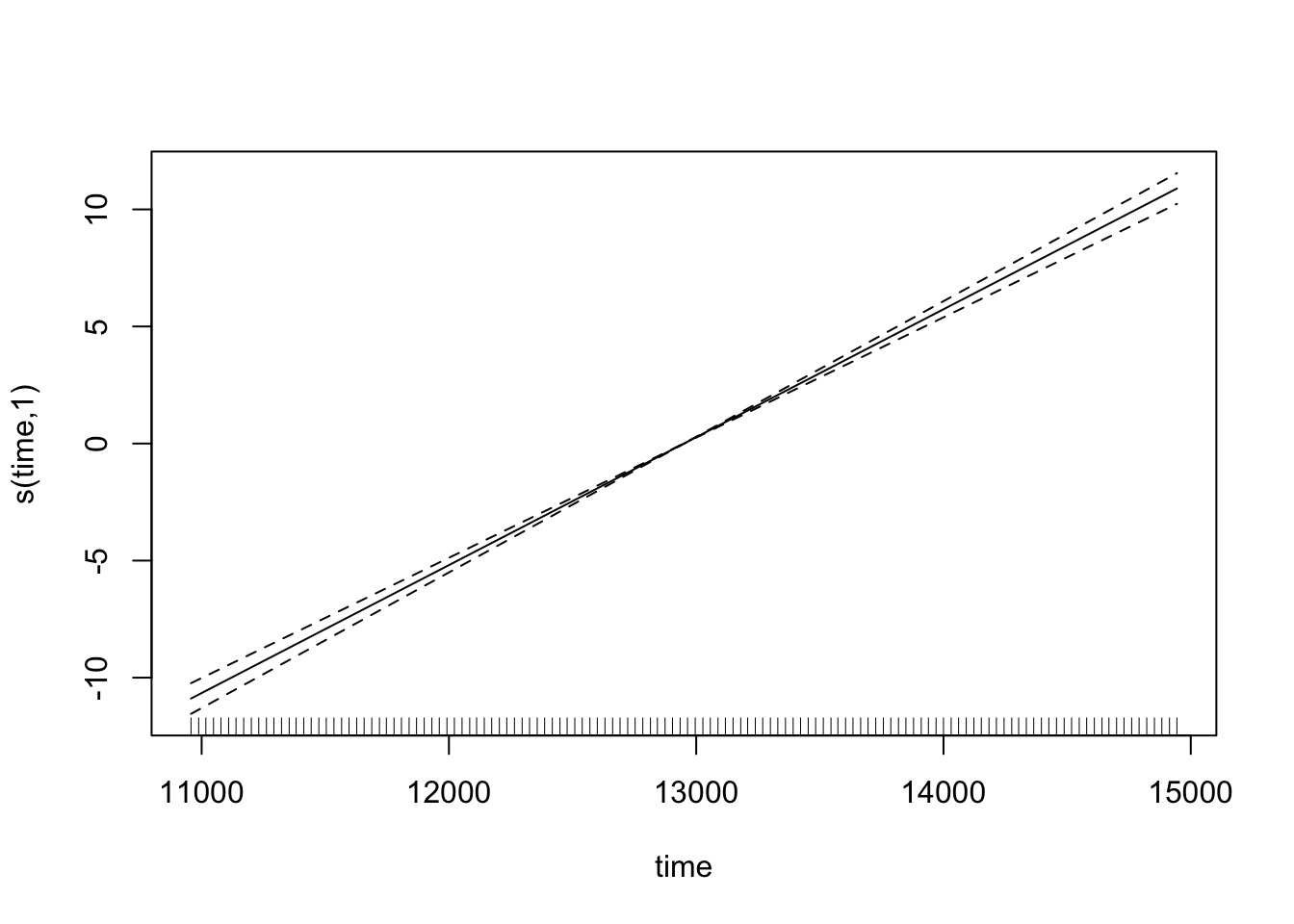
Note how the smooth term actually reduces to a ‘normal’ linear term here (with an edf of 1) - that’s the nice thing about penalised regression splines. But if we check the model, then we see something is amuck.
par(mfrow = c(2, 2))
gam.check(CO2_time)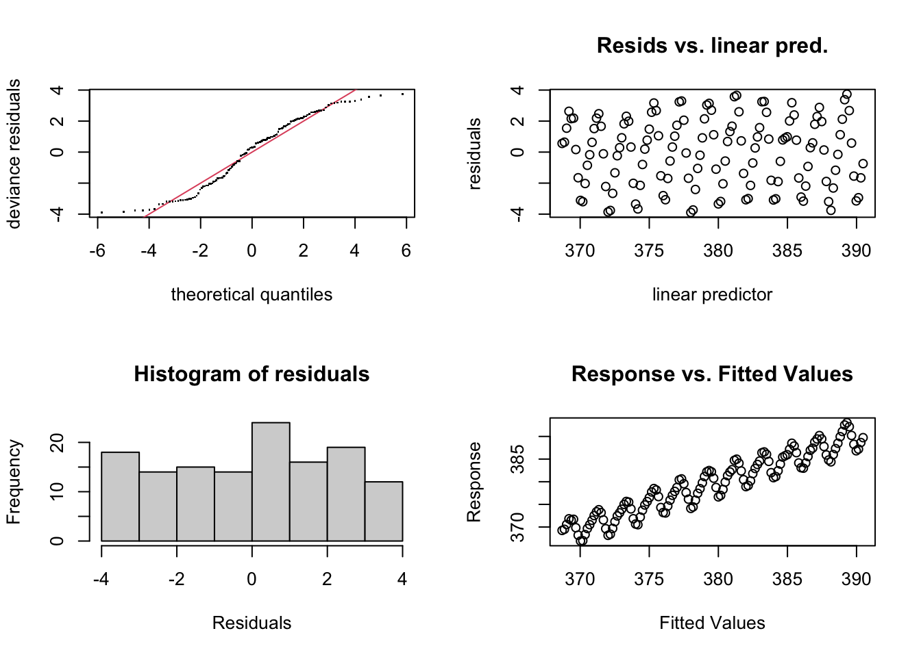
The residual plots have a very odd looking rise-and-fall pattern - clearly there is some dependance structure (and we can probably guess it has something to do with intra-annual fluctuations). Let’s try again, and introduce something called a cyclical smoother. \[y = \beta_0 + f_{\mathrm{intrannual}}(month) + f_{\mathrm{trend}}(time) + \varepsilon, \quad \varepsilon \sim N(0, \sigma^2)\] The cyclical smooth term, \(f_{\mathrm{intrannual}}(month)\), is comprised of basis functions just the same as we have seen already, except that the end points of the spline are constrained to be equal - which makes sense when we’re modelling a variable that is cyclical (across months/years).
We’ll now see the bs = argument to choose the type of smoother, and the k = argument to choose the number of knots, because cubic regression splines have a set number of knots. We use 12 knots, because there are 12 months.
CO2_season_time <- gam(co2 ~ s(month, bs = "cc", k = 12) + s(time), data = CO2, method = "REML")Let’s look at the fitted smooth terms:
par(mfrow = c(1, 2))
plot(CO2_season_time)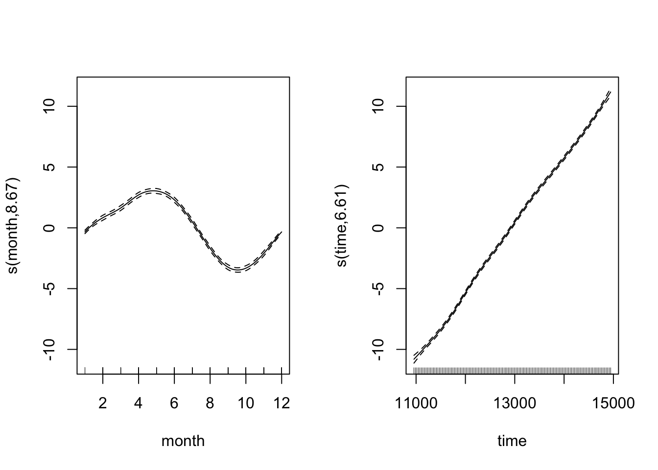
Looking at both smooth terms, we can see that the monthly smoother is picking up that monthly rise and fall of CO\(_2\) - looking at the relative magnitudes (i.e. monthly fluctuation vs. long-term trend), we can see how important it is to disintangle the components of the time series. Let’s see how the model diagnostics look now:
par(mfrow = c(2, 2))
gam.check(CO2_season_time)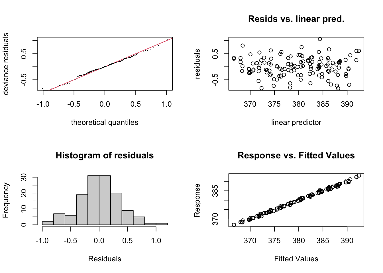
Much better. Let’s look at how the seasonal component stacks up against the full long term trend.
CO2_season_time <- gam(co2 ~ s(month, bs = "cc", k = 12) + s(time), data = CO2_dat, method = "REML")
par(mfrow = c(1, 2))
plot(CO2_season_time)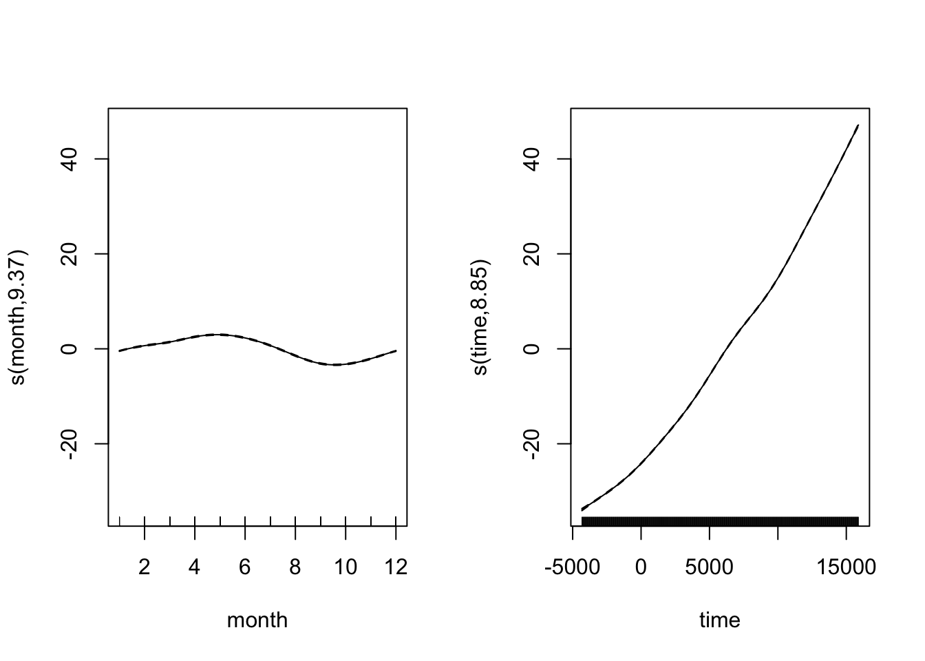
There’s more to the story - pephaps spatial autocorrelations of some kind? gam can make use of the spatial autocorrelation structures available in the nlme package, more on that next time. Hopefully for the meantime GAMs now don’t seem qutie so scary or magical, and you can start to make use of what is really an inrecibly flexible and powerful modelling framework.
Communicating the results
You can essentially present model results from a GAM as if it were any other linear model, the main difference being that for the smooth terms, there is no single coefficient you can make inference from (i.e. negative, positive, effect size etc.). So you need to rely on either interpretting the parital effects of the smooth terms visually (e.g. from a call to plot(gam_model)) or make inference from the predicted values. You can of course include normal linear terms in the model (either continuous or categorical, and in an ANOVA type framework even) and make inference from them like you normally would. Indeed, GAMs are often useful for accounting for a non-linear phenomonon that is not directly of interest, but needs to be acocunted for when making inferece about other variables.
You can plot the partial effects by calling the plot function on a fitted gam model, and you can look at the parametric terms too, possibly using the termplot function too. You can use ggplot for simple models like we did earlier in this tutorial, but for more complex models, it’s good to know how to make the data using predict. We just use the existing time-series here, but you would generate your own data for the newdata= argument.
CO2_pred <- data.frame(
  time = CO2_dat$time,
  co2 = CO2_dat$co2,
  predicted_values = predict(CO2_season_time, newdata = CO2_dat)
)
ggplot(CO2_pred, aes(x = time)) +
  geom_point(aes(y = co2), size = 1, alpha = 0.5) +
  geom_line(aes(y = predicted_values), colour = "red")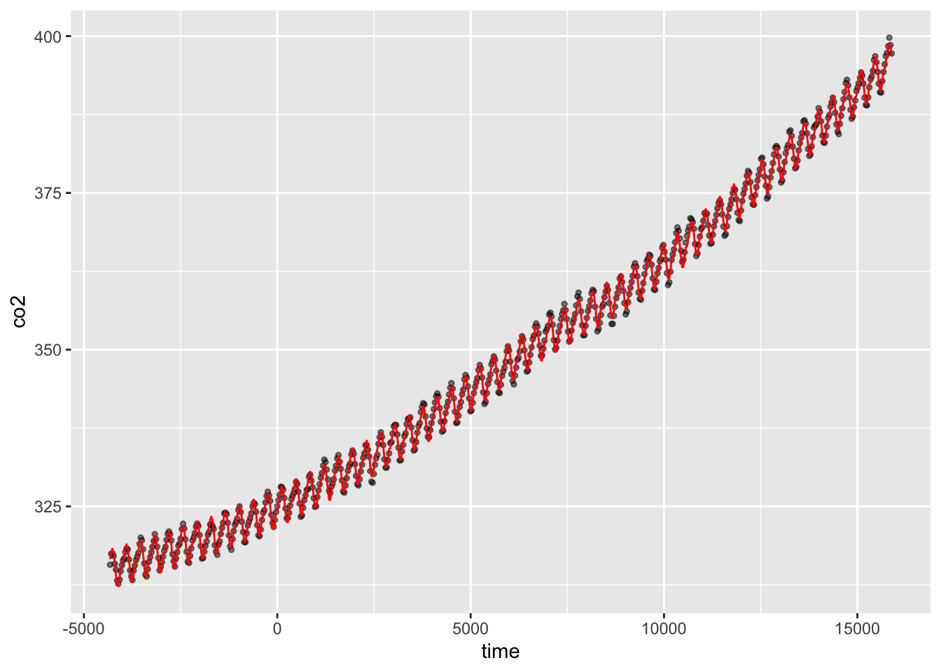
Further help
The R help ?gam is very good, and there is masses of information to read
Check out ?gamm, ?gamm4 and ?bam
Use citation("mgcv") for a range of papers with more technical explanations - the book on GAMs with R is particularly good (there’s a 2017 version)
A great blog with lots of stuff on GAMs: https://www.fromthebottomoftheheap.net/
Author: Mitchell Lyons
Year: 2017
Last updated: Feb 2022