Introduction and Binary Data
Introduction and binomial data
Linear models (e.g., linear regression) are used to model the relationship between a continuous response variable \(y\) and one or more explanatory variables \(x_1, x_2, \cdots\). When we have a discrete response we use generalised linear models (GLM’s).

For example, if had surveyed a beach and wanted to analyse how the presence of a crab varied with time and distance from the water line, the response variable is discrete: the presence or absence of a crab in a given replicate. The first few rows of the data set would look like this:
##   X Dist Time CrabPres
## 1 1    0    5        0
## 2 2    0    5        1
## 3 3    0    5        1
## 4 4    0    5        0
## 5 5    0    5        0
## 6 6    2    5        0
Properties of GLM’s. Discrete response data, like counts and presence/absence data, generally exhibit a mean-variance relationship. For example; for counts that are on average 5, we would expect most samples to be between about 1 and 9, but for counts that are on average 500, most of the observations will tend to be between 450 and 550, giving us a much larger variance when the mean is large.
Linear models assume constant variance. You might have learned to transform count data and then fit a linear model. This can reduce the mean variance relationship, but it won’t get rid of it completely, especially if you have a lot of zeros in your data. To analyse discrete data accurately we need to use GLM’s.
A GLM makes some important assumptions (we’ll check these later for our examples)
- The observed \(y\) are independent, conditional on some predictors \(x\)
- The response \(y\) come from a known distribution with a known mean-variance relationship
- There is a straight line relationship between a known function \(g\) of the mean of \(y\) and the predictors \(x\)
\[ g(\mu_y) = \alpha + \beta_1 x_1 + \beta_2 x_2 + \cdots \]
Note: link functions g() are an important part of fitting GLM’s, but beyond the scope of this introductory tutorial. All you need to know is that the default link for binomial data is the logit() and for count data it’s log(). For more information see ?family.
Running the analysis
Binomial data
First, we will show you how to fit a model to binomial data, i.e., presence/absence data or data as 0/1. Fitting GLM’s uses very similar syntax to fitting linear models. We use the glm function instead of lm. We also need to add a ?family argument to specify whether your data are counts, binomial etc.
For this worked example, download the sample data set on the presence and absence of crabs on the beach, Crabs.csv and import into R.
Crab_PA <- read.csv("Crabs.csv", header = T)To test whether the probability of crab presence changes with time (a factor) and distance (a continuous variable), we fit the following model. The response variable (presence/absence of crabs) is binomial, so we use family=binomial.
ft.crab <- glm(CrabPres ~ Time * Dist, family = binomial, data = Crab_PA)Assumptions to check
Before we look at the results of our analysis it’s important to check that our data met the assumptions of the model we used. Let’s look at all the assumptions in order.
Assumption 1 : The observed \(y\) are independent, conditional on some predictors \(x\)
We can’t check this assumption from the results, but you can ensure it’s true by taking a random sample for your experimental design. If your experimental design involves any pseudo-replication, this assumption will be violated. For certain types of pseudo-replication you can use mixed models instead.
Assumption 2 : The response \(y\) come from a known distribution with a known mean-variance relationship
The mean variance relationship is the main reason we use GLM’s instead of linear models. We need to check that the distribution models the mean-variance relationship of our data well. For binomial data this is not a big concern, but later on when we analyse count data it’ll be very important. To check this assumption we look at a plot of residuals, and try to see if there is a fan shape.
plot(ft.crab, which = 1)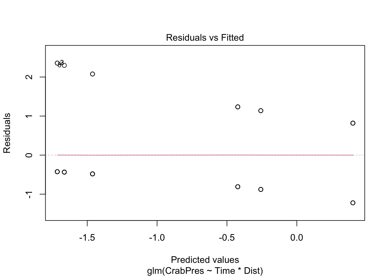
Unfortunately the glm plot function gives us a very odd looking plot due to the discreteness of the data (i.e., many points on top of each other).
For a more useful plot we can instead fit the model using the manyglm function in the mvabund package. We need a slight change to the family argument, for manyglm we write family = "binomial".
library(mvabund)
ft.crab.many <- manyglm(CrabPres ~ Time * Dist, family = "binomial", data = Crab_PA)
plot(ft.crab.many)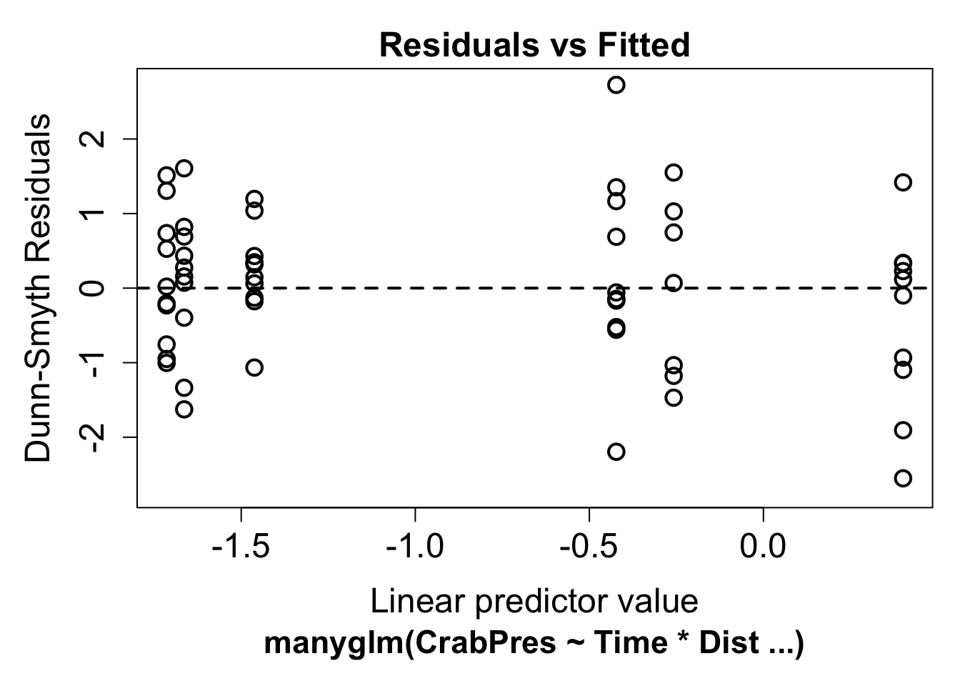
Now we can look for a fan shape in the residual plot. For these data, there doesn’t seem to be a fan shape, so we can conclude the mean-variance assumption the model made was reasonable for our data. The residuals in this plot have a random component. If you see a pattern it’s best to repeat the plot a few times to see if the pattern is real.
Assumption 3 : There is a straight line relationship between a known function \(g\) of the mean of \(y\) and the predictors \(x\)
To check this assumption, we check the residual plot above for non-linearity, or a U-shape. In our case there is no evidence of non-linearity. If the residuals seem to go down then up, or up then down, we may need to add a polynomial function of the predictors using the poly function.
Interpreting the results
If all the assumption checks are okay, we can have a look at the results the model gave us. The two main functions for inference are the same as for linear models: summary and anova.
The p-values these give you if you use glm for fitting the model work well in large samples, although they are still approximate. For binomial models in particular the p-values from the summary function can be funny, and we prefer to use the anova function to see if predictors are significant. The summary() function is still useful to look at the model equation.
anova(ft.crab, test = "Chisq")## Analysis of Deviance Table
##
## Model: binomial, link: logit
##
## Response: CrabPres
##
## Terms added sequentially (first to last)
##
##
## Df Deviance Resid. Df Resid. Dev Pr(>Chi)
## NULL 56 71.097
## Time 1 6.6701 55 64.427 0.009804 **
## Dist 1 0.7955 54 63.631 0.372448
## Time:Dist 1 0.1647 53 63.466 0.684852
## ---
## Signif. codes: 0 '***' 0.001 '**' 0.01 '*' 0.05 '.' 0.1 ' ' 1The p-value for Time is small (P<0.01), so we conclude there is an effect of time on the presence of crabs, but no effect of distance or an interaction between time and distance. This sample is reasonably large, so these p-values should be a good approximation. For a small sample it is often better to use resampling to calculate p-values. When you use manyglm the summary and anova functions use resampling by default.
anova(ft.crab.many)## Time elapsed: 0 hr 0 min 0 sec## Analysis of Deviance Table
##
## Model: CrabPres ~ Time * Dist
##
## Multivariate test:
## Res.Df Df.diff Dev Pr(>Dev)
## (Intercept) 56
## Time 55 1 6.670 0.011 *
## Dist 54 1 0.795 0.370
## Time:Dist 53 1 0.165 0.700
## ---
## Signif. codes: 0 '***' 0.001 '**' 0.01 '*' 0.05 '.' 0.1 ' ' 1
## Arguments: P-value calculated using 999 iterations via PIT-trap resampling.In this case the results are quite similar, but in small samples it can often make a big difference.
You can also use summary with either the glm or manyglm function. This is interpreted in a similar manner as for linear regression, but we need to include the link function, g.
summary(ft.crab)##
## Call:
## glm(formula = CrabPres ~ Time * Dist, family = binomial, data = Crab_PA)
##
## Deviance Residuals:
## Min 1Q Median 3Q Max
## -1.3518 -0.6457 -0.5890 1.0125 1.9390
##
## Coefficients:
## Estimate Std. Error z value Pr(>|z|)
## (Intercept) -3.00604 1.47469 -2.038 0.0415 *
## Time 0.25835 0.17439 1.481 0.1385
## Dist -0.03193 0.23923 -0.133 0.8938
## Time:Dist 0.01143 0.02830 0.404 0.6863
## ---
## Signif. codes: 0 '***' 0.001 '**' 0.01 '*' 0.05 '.' 0.1 ' ' 1
##
## (Dispersion parameter for binomial family taken to be 1)
##
## Null deviance: 71.097 on 56 degrees of freedom
## Residual deviance: 63.466 on 53 degrees of freedom
## AIC: 71.466
##
## Number of Fisher Scoring iterations: 4If \(p\) is the probability of crab presence, this output tells us
\[ logit(p) = -3.01 + 0.26 \times \text{Time} -0.03 \times \text{Dist} +0.01 \times \text{Time} \times \text{Dist}\]
Communicating the results
Results of GLM’s are communicated in the same way as results for linear models. For one predictor it suffices to write one line, e.g., “There is strong evidence that the presence of crabs varies with time (p = 0.01). For multiple predictors it’s best to display the results in a table. You should also indicate which distribution was used (e.g. Binomial for presence/absence, Poisson or negative-binomial for counts) and if resampling was used for inference.
Further help
You can type ?glm and ?manyglm into R for help with these functions.
Faraway, JJ. 2005. Extending the linear model with R: generalized linear, mixed effects and nonparametric regression models. CRC press.
Zuur, A, EN Ieno and GM Smith. 20074. Analysing ecological data. Springer Science & Business Media, 2007.
More advice on interpreting coefficients in glms
Author: Gordana Popovic
Year: 2016
Last updated: Feb 2022