Simple Maps with ggmap
Being able to make a simple map is a very useful skill for all sorts of applications. Here, we will introduce some of the basics of working with spatial data, and use R to produce simple and easy maps. You could use the same technique to make a map for a presentation, or a figure for a report or publication.
There are many packages that are useful for plotting and manipulating spatial data in R. For simplicity, we’re going to solely use the package ggmap for this exercise. To get started, install this package and load into R.
library(ggmap)Setting up ggmap
The ggmap package “makes it easy to retrieve raster map tiles from popular online mapping services like Google Maps and Stamen Maps and plot them using the ggplot2 framework”.
To use the package you’ll need to setup an API key to google maps. For information on how to do this see the package homepage on GitHub. An alternative interface to OpenStreetMap can also be used with slightly different functions.
Making your first map
In this example, let’s say we collected data from five sites near Royal National Park in New South Wales, Australia, and want to display the locations we visited.
Using the function get_map, we can download an image from Google maps at any named location:
basemap <- get_map("Royal National Park", zoom = 12)and then plot it with the function ggmap:
ggmap(basemap)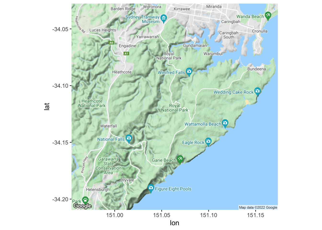
The argument of get_map is simply any place searchable on Google Maps (in this case ‘Royal National Park’) - easy!
To add point data for our five survey sites, we first need to make a new data frame holding the place name, latitude and longitude of each site (or import this data from a spreadsheet).
ptdata <- data.frame(
  "PlaceName" = c(
    " Hacking R. ", " Cabbage Tree Ck. ",
    " Marley Ck. ", " Wattamolla Ck. ",
    " Waratah R. "
  ),
  "Long" = c(
    151.054823, 151.124566, 151.139216,
    151.115645, 150.960431
  ),
  "Lat" = c(
    -34.074918, -34.090796, -34.111972,
    -34.136046, -34.172308
  )
)
We can add these points to our map based on the Latitude (y) and Longitude (x) coordinates. It is important that the points and the other features on the map work on the same scale - or ‘projection’. These locations were estimated from Google Maps data for this reason - estimate your own via LatLong.net).
ggmap(basemap) + geom_point(data = ptdata, aes(x = Long, y = Lat))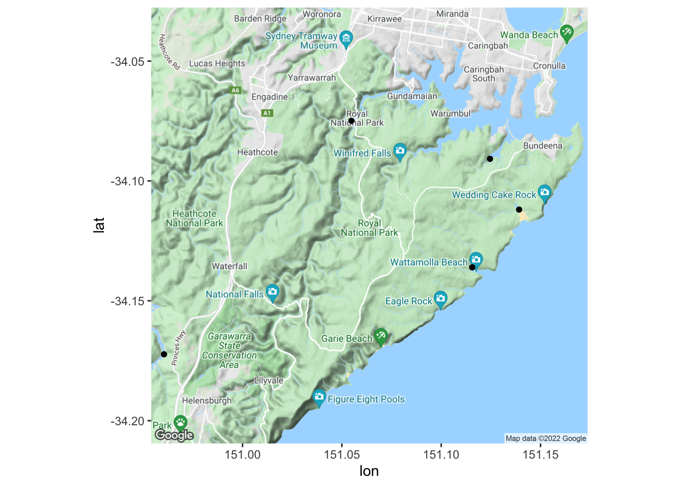
Well done -you made your first map with R! Easy! You may have noticed that ggmap uses familiar graphics code from the package ggplot (see plotting with ggplot).
Making a presentation-ready map
By tweaking a few options, we can make this look more suitable for a presentation.
First, adjust some of the options in get_map:
- use
boundto choose the extent/bounding box of the map. Here, we are using the minimum and maximum values of latitude and longitude from our site coordinates - try
maptype = "hybrid"to see the satellite imagery and roads data
- increase the
zoomlevel to improve detail
bound <- c(
  left = min(ptdata$Long) - 0.05, bottom = min(ptdata$Lat) - 0.05,
  right = max(ptdata$Long) + 0.05, top = max(ptdata$Lat) + 0.05
)
Pres_basemap <- get_map(bound, zoom = 11, maptype = "hybrid")Second, adjust some of the options for plotting:
geom_point tweaks for the dots at each site location:
* use colour = "white" to have the points stand out
* use size to change point size
geom_text tweaks for the labels for each site:
- use
sizeto change text size - use
colour = "white"to have the labels stand out - use
hjustandvjustadjust the horizontal and vertical position of labels
- use
labsto define the x and y axis labels
ggmap(Pres_basemap) +
  geom_point(
    data = ptdata, aes(x = Long, y = Lat),
    colour = "white"
  ) +
  geom_text(
    data = ptdata,
    aes(x = Long, y = Lat, label = PlaceName),
    size = 4,
    colour = "white",
    hjust = "inward"
  ) +
  labs(x = "Longitude", y = "Latitude")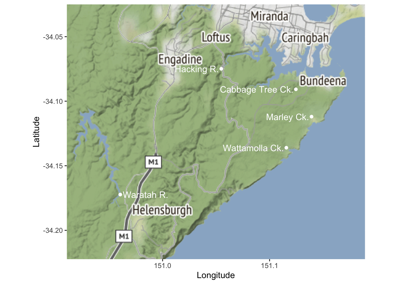
Making a publication-ready map
For a paper or report, you probably want a simpler black and white map.
- use
boundto set the extent as above
- try
get_stamenmapto get an austere basemap (eg. Stamen “toner-lite”)
- use
theme_bw()from ggplot to get a stripped-back theme
Pub_basemap <- get_stamenmap(bound, zoom = 13, maptype = "toner-lite")ggmap(Pub_basemap) +
geom_point(data = ptdata, aes(x = Long, y = Lat, label = PlaceName)) +
geom_text(
data = ptdata,
aes(x = Long, y = Lat, label = PlaceName),
size = 4,
fontface = "bold",
hjust = "right"
) +
theme_bw() +
theme(axis.title = element_blank())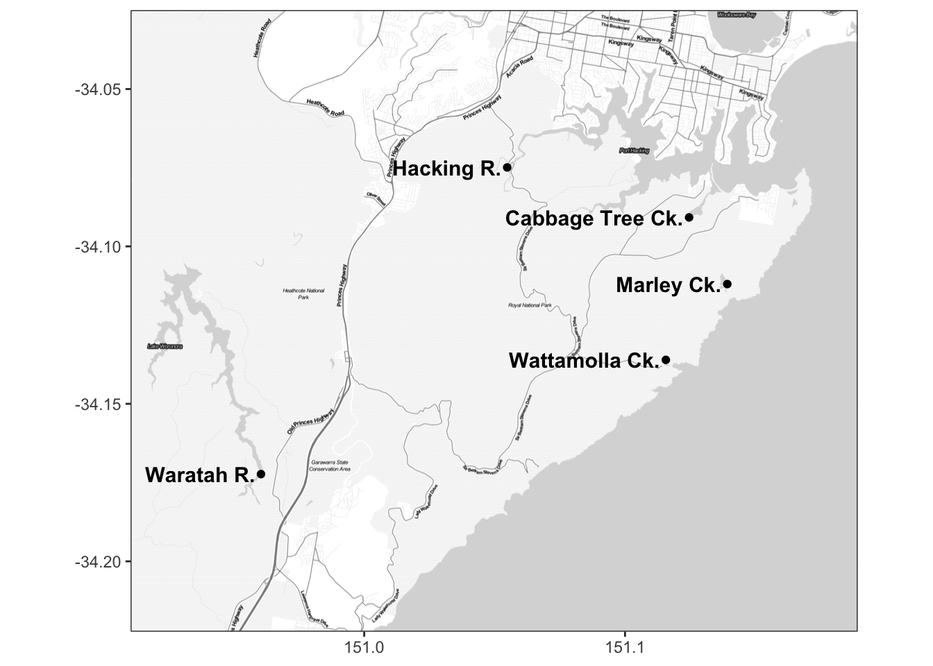
Further help
Read the ggmap documentation for more examples and ideas.
ggmap cheat sheet from the National Centre for Ecological Analysis and Synthesis.
Author: Kingsley Griffin, edits by Daniel Falster
Year: 2017
Last updated: Feb 2022