Two Sample T-test
An independent samples t-test aka a two sample t-test is one of the most commonly used statistical tests. It is used for comparing whether the means of two samples are statistically different from each other (e.g., control vs. treatment, site A vs site B etc). For example, consider the simple case of whether a sample of pH measurements from one river differs from a sample of pH measurements from a second river.

The null hypothesis is that the population means from which the two samples are taken are equal \[H_o: \mu_1=\mu_2\].
The test statistic, t, is:
\[t = \frac{\bar{x_{1}}-\bar{x_{2}}}{s_{\bar{y_{1}}-\bar{y_{2}}}}\]
where the denominator is the standard error of the difference between the two means.
\[\sqrt{\frac{(n_{1}-1)s_{1}^{2}+(n_{2}-1)s_{2}^{2}}{n_{1}+n_{2}-2}{(\frac{1}{n_{1}}}+\frac{1}{n_{2}})}\]
Note that the size of test statistic depends on two things: 1) how different the two means are (the numerator) and 2) how much variation is present within each sample (the denominator).
This equation is for the pooled variance t-test. For a separate variances t-test (also known as Welch’s t test), which does not assume equal variances, the denominator is:
\[\sqrt{\frac{s_1^2}{n_1}+\frac{s_2^2}{n_2}}\]
Note that a t test is a special case of a linear model with a single continuous response variable and a single categorical predictor variable that has two levels.
Running the analysis
An independent samples t-test can be run with the same t.test function as used for one sample or paired t-tests. For an independent samples t-test assuming equal variances, we would use:
t.test(x <- my_sample1, y = my_sample2, var.equal = TRUE)where my_sample1 and my_sample2 are vectors containing the measurements from each sample.
More commonly, we would use a data frame with the response and predictor variables as separate columns. You can then use a formula statement, y ~ x, to specify the response and predictor variables rather than the code above. Consider the simple example where you wanted to compare the pH of two rivers. Ten replicate pH measures were taken from each river.
Download the sample data set, River_pH.csv, and import into R.
River_pH <- read.csv(file = "River_pH.csv", header = TRUE)The t-test is run with the t.test function, with the arguments specifying the response variable (pH) to the left of the ~, the predictor variable (River_name) to the right of the ~, and the data frame to be used.
t.test(pH ~ River_name, data = River_pH, var.equal = TRUE)The argument var.equal = TRUE specifies that we are assuming equal variances. Note the default t-test argument for the alternative hypothesis is a two-tailed test. If you want to conduct a one-tailed test you must add an argument to the function specifying alternative = "greater" or alternative = "less".
Interpreting the results
##
##  Two Sample t-test
##
## data:  River_pH$pH by River_pH$River_name
## t = 6.9788, df = 18, p-value = 1.618e-06
## alternative hypothesis: true difference in means between group A and group B is not equal to 0
## 95 percent confidence interval:
##  1.574706 2.931168
## sample estimates:
## mean in group A mean in group B
##        8.661497        6.408560
The output of a t-test is straight-forward to interpret. In the above output, the test statistic t = 6.9788 with 18 degrees of freedom, and a very low p value (p < 0.001). We can therefore reject the null hypothesis that the two rivers have the same pH.
You also get the means from the two samples (needed to know which one is larger if the test is significant), and the 95% confidence interval for the difference between the two means (this will not overlap zero when the test is signficant).
Assumptions to check
t-tests are parametric tests, which implies we can specify a probability distribution for the population of the variable from which samples were taken. Parametric (and non-parametric) tests have a number of assumptions. If these assumptions are violated we can no longer be sure that the test statistic follows a t distribution, in which case p-values may be inaccurate.
Normality. The data are normally distributed. Note however that t tests are reasonably robust to violations of normality (although watch out for the influence of outliers).
Equal variance. The variances of each sample are assumed to be approximately equal. t tests are also reasonably robust to violations of equal variance if sample sizes are the same but can be problematic when sample sizes are very different.
In the event of unequal variances, it may be better to perform a Welch’s t test which does not assume equal variances. To conduct a Welch test in R, the var.equal argument in t.test function should be changed to var.equal=FALSE. This is in fact the default argument for t.test if not specified.
Independence. The observations should have been sampled randomly from the population so that the two sample means are unbiased estimates of the population means. If individual replicates are linked in any way, then the assumption of independence will be violated.
Communicating the results
Written. As a minimum, the observed t statistic, the P-value and the number of degrees of freedom should be reported. For example, you could write “the pH was significantly higher in River A than River B (independent samples t-test: t = 6.98, df = 18, P < 0.001)”.
Visual. Box plots or column graphs with error bars are effective ways of communicating the variation in a single continuous response variable versus a single categorical predictor variable.
boxplot(pH ~ River_name, data = River_pH, xlab = "River name", ylab = "pH")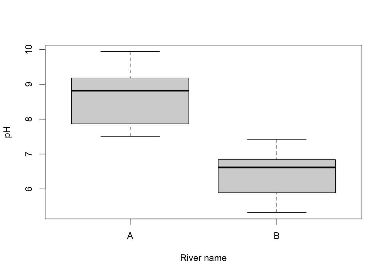
Further help
Type ?t.test to get the R help for this function.
Quinn and Keough (2002) Experimental design and data analysis for biologists. Cambridge University Press. Chapter 3: Hypothesis testing.
McKillup (2012) Statistics explained. An introductory guide for life scientists. Cambridge University Press. Chapter 9: Comparing the means of one and two samples of normally distributed data.
Author: Alistair Poore
Year: 2016
Last updated: Feb 2022